Chapter 2 Summary statistics and distributions
2.1 Introduction
Understanding a data set involves summarizing it so that you can better understand its characteristics. In combination with graphing and visualizing data, this chapter will complete our understanding of descriptive statistics.
This chapter will discuss descriptive statistics such as measures of central tendency (e.g., the mean, median, and mode), spread, (e.g., the variance and standard deviation), and position (e.g., quartiles and outliers). These values are often reported in final reports to convey the properties of data. We will round out the chapter by discussing distributions and random variables, numerical variables that describe the outcomes of a chance process. This will lead us into discussing probability in subsequent chapters.
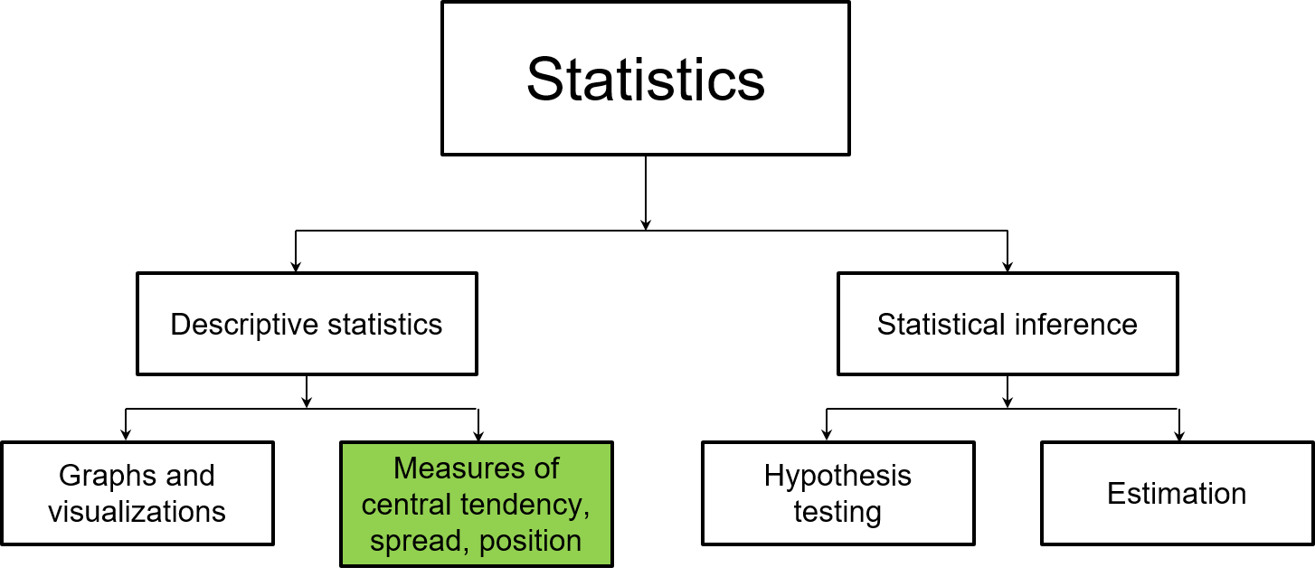
FIGURE 2.1: This chapter focuses on how summary statistics are used in descriptive statistics.
2.2 Summary statistics
A statistic can be defined as a summary of a sample. In contrast, a parameter represents a population constant. This section will discuss the common statistics we can calculate from samples. When we begin discussing random variables in the next section, you will begin to see how statistics are related to parameters.
2.2.1 Measures of central tendency
When a colleague mentions she calculated “the average” of a value, she is referring to a measure of central tendency. Measures of central tendency include the mean, median and mode.
The mean, denoted by \(\bar{x}\), is calculated by summing all values and dividing by the number of values \(n\):
\[{\bar{x} = \frac {\sum_{i=1}^{n} x_i}{n}} = \frac{x_1 + x_2 + ... + x_n}{n}\] The median is determined by finding the middle value of a sorted data set. The median is located in the (n+1)/2 position. The median is considered a resistant central tendency measure because compared to the mean, the median is not impacted by extreme values.
The mode is defined as the measurement that occurs most frequently. There are pros and cons to using these measures of central tendency, as indicated in Table 2.1.
| Statistic | Pros | Cons |
|---|---|---|
| Mean | Most widely used in natural sciences | Affected by extreme values |
| Median | Not affected by extreme values; useful for skewed distributions | Does not take into account precise values |
| Mode | Effective if used with qualitative data | May not exist; can be more than one mode; may not be representative of the average for small samples. |
As an example, we will determine various measures of central tendency on the number of chirps that a striped ground cricket makes. Ecologists believe that the number of chirps a striped ground cricket makes every second is related to the air temperature.
The data are from Pierce (1943) and contain the number of chirps per second (cps) and the air temperature, measured in degrees Fahrenheit (temp_F). The chirps data set from the stats4nr package contains the 15 observations of chirps per second:
library(stats4nr)

head(chirps)
## # A tibble: 6 x 2
## cps temp_F
## <dbl> <dbl>
## 1 20 93.3
## 2 16 71.6
## 3 19.8 93.3
## 4 18.4 84.3
## 5 17.1 80.6
## 6 15.5 75.2We can calculate the mean by hand for the number of chirps per second:
\[{\bar{x} = \frac{20.0 + 16.0 + ... + 14.4}{15} = 16.65}\]
The median can be found by sorting the cps variable with the arrange() function. The median is located in the (15+1)/2 = 8th position:
chirps %>%
  arrange(cps)
## # A tibble: 15 x 2
## cps temp_F
## <dbl> <dbl>
## 1 14.4 76.3
## 2 14.7 69.7
## 3 15 79.6
## 4 15.4 69.4
## 5 15.5 75.2
## 6 16 71.6
## 7 16 80.6
## 8 16.2 83.3
## 9 17 73.5
## 10 17.1 80.6
## 11 17.1 82
## 12 17.2 82.6
## 13 18.4 84.3
## 14 19.8 93.3
## 15 20 93.3The median chirps per second is 16.2. If the number of observations were even, we would calculate the average of the two middle observations in the sorted list. Fortunately, R has two built-in functions to calculate the mean and median:
mean(chirps$cps)## [1] 16.65333median(chirps$cps)## [1] 16.2Unfortunately, R does not have a built-in function to calculate a mode. Fortunately, the modeest package (Poncet 2019) contains the mfv() function, which returns the most frequent value (or values) in a numerical variable:
install.packages("modeest")

library(modeest)

mfv(chirps$cps)
## [1] 16.0 17.1We see that there are two modes for the number of chirps per second: 16.0 and 17.1. These values are similar in magnitude to the mean and median.
2.2.2 Measures of spread
Aside from understanding the average of the data, or its signal, it is also informative to characterize how spread out the data are, or its noise. For example, the range, defined as the minimum subtracted from the maximum value, is a useful representation of how noisy the data are. The range is a quick measure of spread to calculate but is also very sensitive to extreme values.
The variance measures the average squared distance of the observations from their mean. To calculate the sample variance \(s^2\), the average of the squared distance is determined:
\[{s^2 = \frac {1}{n-1} {\sum_{i=1}^{n} (x_i- \bar{x})^2}} = \frac {1}{n-1} {(x_1- \bar{x})^2 + (x_2- \bar{x})^2 + ... + (x_n- \bar{x})^2}\]
While the variance is used widely in statistics, it is not always a meaningful number to characterize a variable of interest. This is because its units are squared. For example, we’ll calculate the variance of the cps variable in the chirps data set:
\[{s^2 = \frac {1}{15-1} {(20.0 - 16.65)^2 + (16.0 - 16.65)^2 + ... + (14.4 - 16.65)^2}} = 2.90\]
The calculation indicates that the variance is 2.90 squared chirps per second. For a more useful number, instead we’ll take the square root of the variance and report the standard deviation, defined as the average distance of the observations from their mean:
\[{s} = \sqrt{s^2}\]
The standard deviation for cps is then:
\[{s} = \sqrt{2.90} = 1.70\]
Now, the calculation indicates that the standard deviation is 1.70 chirps per second, a more informative number to describe our data. The standard deviation is the most common measure of spread used in natural resources disciplines.
The variance (var()) and standard deviation (sd()) functions are calculated as:
var(chirps$cps)## [1] 2.896952sd(chirps$cps)## [1] 1.702044Another measure of spread is the coefficient of variation (CV), a widely used statistic that “standardizes” the standard deviation relative to its mean. If we were only to look at the standard deviation of two different variables, their magnitudes might be vastly different. However, by standardizing the two variables we can compare how variable each is relative to its mean value. The CV is always expressed as a percent:
\[{CV = \frac {s}{\bar x}\times100}\] The CV for the chirps data then is:
\[{CV = \frac {1.70}{16.65}\times100 = 10.22 \%}\]
A CV of 10.33% is relatively low when investigating biological and environmental data. For comparison, most variables measured in a forest setting, such as tree diameters and volume, have CVs around 100% (Freese 1962). In R, the standard deviation and mean can be combined in a single line of code to calculate the CV:
(sd(chirps$cps) / mean(chirps$cps)) * 100## [1] 10.220442.2.3 Measures of position
We are often interested to know how a particular value can be compared to other values in a data set. One value that uses the mean and standard deviation to measure the position of a variable of interest is the z-score. The z-score measures how different the data are from what we would expect (i.e., the mean). We’ll revisit the z-score when we get into hypothesis testing, but a few important things to know include:
- a z-score equal to 0 signals that a value is equal to the mean,
- a z-score less than 0 signals that a value is less than the mean, and
- a z-score greater than 0 signals that a value is greater than the mean.
The value of the z-score tells you how many standard deviations a value \({x_i}\) is away from the mean \({\bar{x}}\). Here, we will compare the value to the sample mean and standard deviation:
\[{z_i = \frac {x_i - \bar{x}}{s}}\]
In the chirps data, a z-score of 0 indicates that the value of interest \(x_i\) is equal to the mean. The figure below shows the corresponding z-scores if the number of chirps per second are 16 and 20, two values that are slightly lower and tremendously greater than the mean. Slightly less than half of observations would be expected to be less than 16. The majority of observations would be expected to be less than 20. In other words, 16 and 20 chirps per second are 0.38 and 1.97 standard deviations away from the mean, respectively.
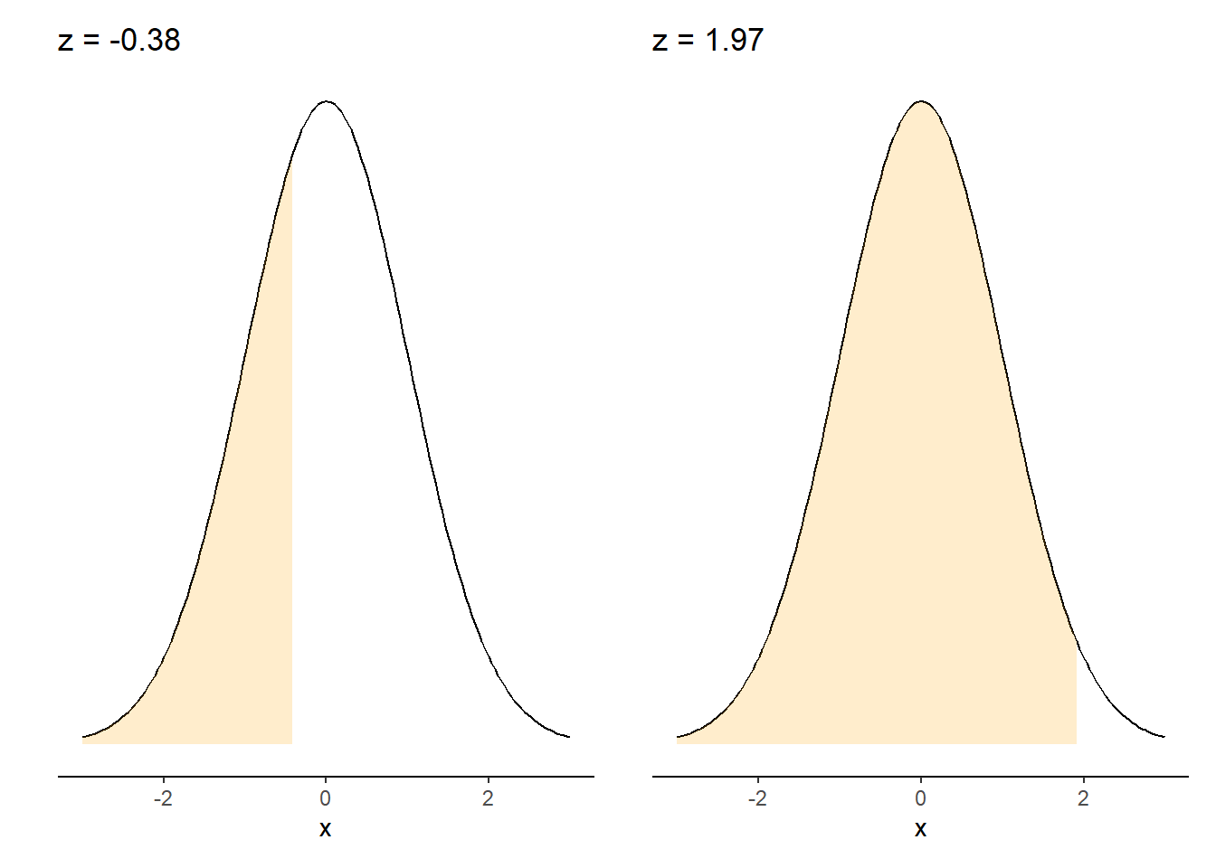
FIGURE 2.2: Z-scores for 16 and 20 chirps per second.
We saw the advantages of a box plot from the last chapter and described how it shows the minimum, first quartile (Q1), median, third quartile (Q3), and maximum values of a variable. Here is a box plot for the chirps per second:
ggplot(data = chirps, aes(x = 1, y = cps)) +
  geom_boxplot() +
  scale_x_continuous(breaks = NULL) +
  labs(y = "Chirps per second")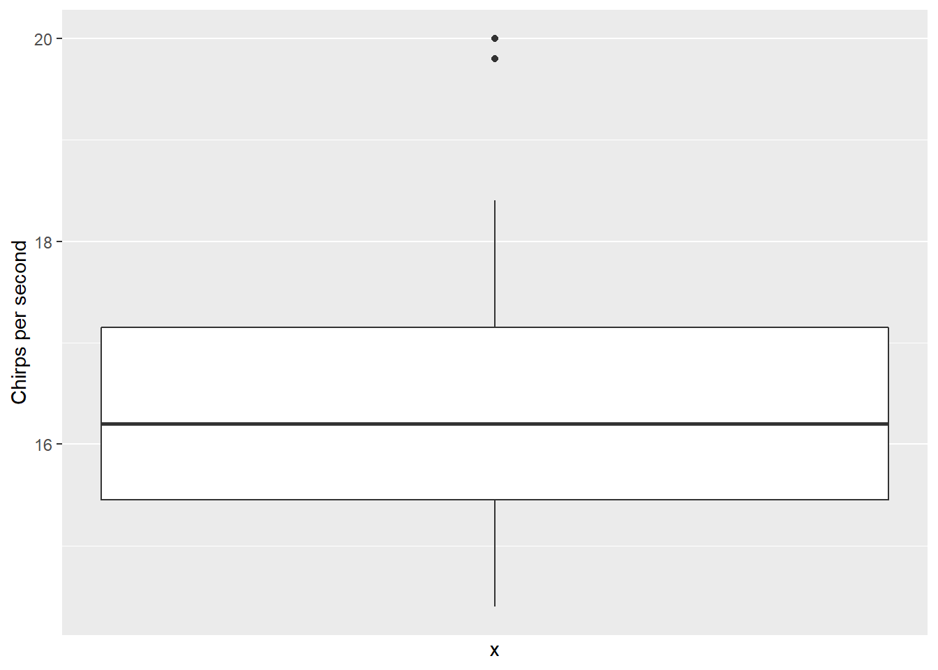
In the box plot, notice that there are two outliers that are shown as points. These correspond to the values at 19.8 and 20.0 chirps per second. By default, the whiskers using geom_boxplot() will extend no more than 1.5 times the interquartile range (IQR), or the difference between Q3 and Q1 on either the lower or upper tail of the distribution. The IQR can be thought of as a range for the middle 50% of data. Hence, the IQR may be preferred over the range because it is less sensitive to extreme values.
The coef = statement can be added within geom_boxplot() to extend the whiskers a greater length from the IQR. For example, we can create a box plot that extends the whiskers to three times the IQR and will “cover up” the outliers:
ggplot(data = chirps, aes(x = 1, y = cps)) +
  geom_boxplot(coef = 3) +
  scale_x_continuous(breaks = NULL) +
  labs(y = "Chirps per second")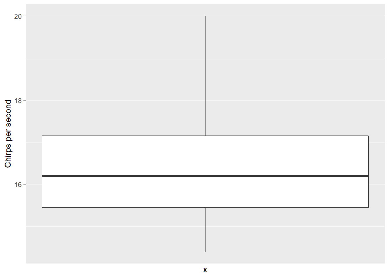
After viewing the box plot, we can also see that the data are right-skewed, because the difference between the maximum value and median is larger than the difference between the minimum value and median. More evidence of a right-skewed distribution is that the median (16.2) is less than the mean (16.65), indicating more large values and makes the mean larger.
DATA ANALYSIS TIP The classification of whether or not an observation is an outlier varies widely by discipline, the kind of instrumentation used, and other characteristics of the data. It is best to always check suspect observations with thorough analysis. Fortunately, after visualizing and summarizing data with descriptive statistics, you are in a great position to identify bad data before you begin your other statistical analyses.
2.2.4 Exercises
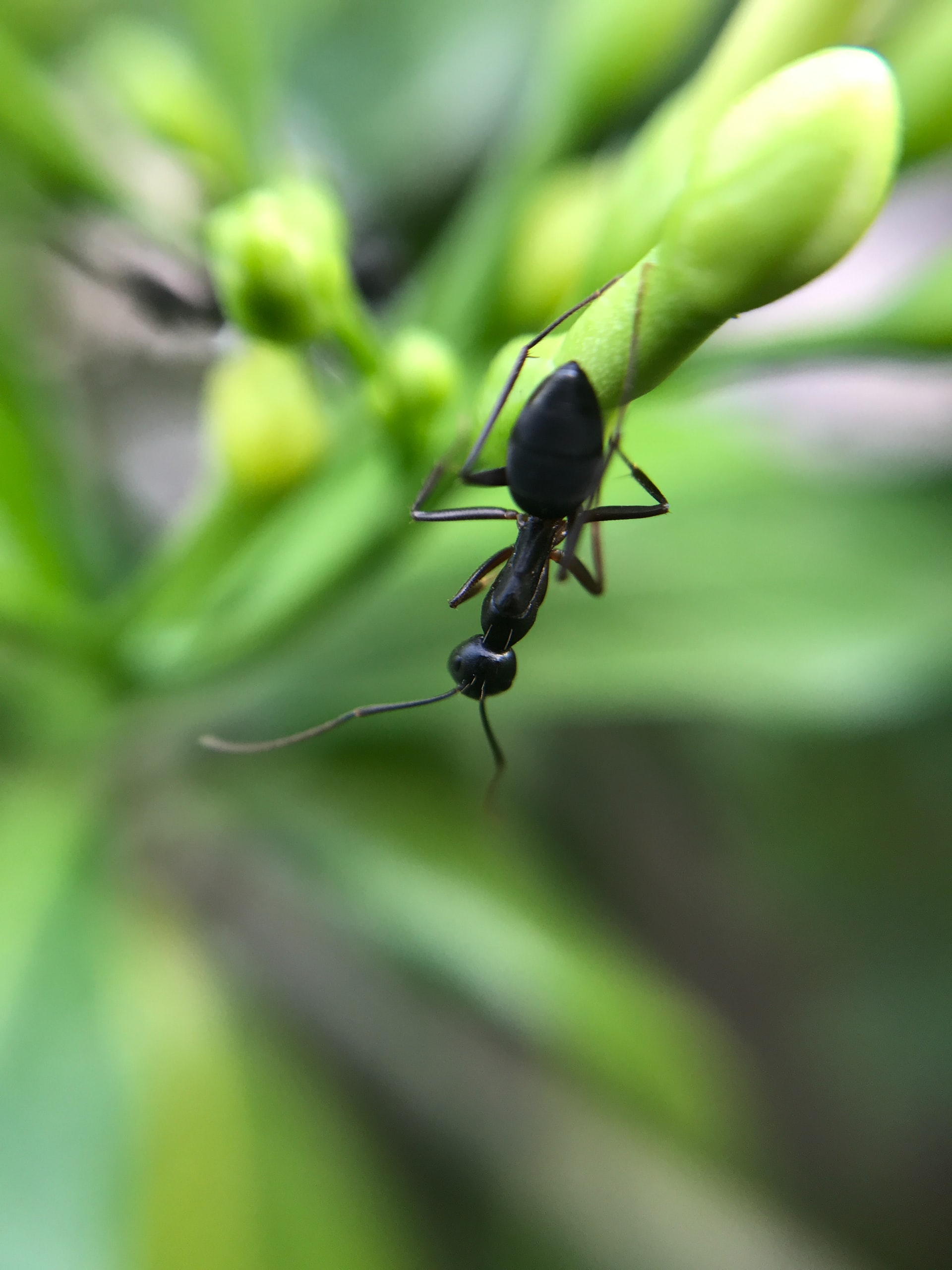
FIGURE 2.3: The following exercises use a dataset on ant species richness. Photo: Unitedbee Clicks on Unsplash.
2.1 Ant species richness was sampled in bogs and forests at 22 sites in Connecticut, Massachusetts, and Vermont, USA (Gotelli and Ellison 2002). Environmental variables in the ant data set from the stats4nr package include species richness at each site by ecotype (forest or bog), latitude (lat), and elevation (elev). The data are contained in the spprich data set. Read in the data set and run the following code to create separate data frames for the two ecosystem types:
library(stats4nr)
head(ant)
## # A tibble: 6 x 5
## site ecotype spprich lat elev
## <chr> <chr> <dbl> <dbl> <dbl>
## 1 TPB Forest 6 42.0 389
## 2 HBC Forest 16 42 8
## 3 CKB Forest 18 42.0 152
## 4 SKP Forest 17 42.0 1
## 5 CB Forest 9 42.0 210
## 6 RP Forest 15 42.2 78forest <- ant %>%
filter(ecotype == "Forest")
bog <- ant %>%
filter(ecotype == "Bog")Use R functions to calculate the mean, median, and mode for the species richness in the forest and bog data sets. Which ecosystem type has a greater mean species richness?
2.2 Create a side-by-side violin plot that shows ant species richness on the x-axis with ecosystem type on the y-axis.
2.3 Learn about and use the range() and IQR() functions to calculate the range and interquartile range for species richness in the forest and bog data sets.
2.4 Calculate the standard deviation and coefficient variation for species richness in the forest and bog data sets. While both measurements reflect a measure of variability, your results will indicate a different answer to the question “Is ant species richness more variable in forests or bogs?” Explain why you obtain different results depending on whether you use the standard deviation or coefficient of variation.
2.5 How many standard deviations away from the mean are 7 species of ants? Write R code to make two calculations: one for the forest and one for the bog data set.
2.6 Instead of using the filter() function to create the forest and bog data sets as we did in exercise 2.1, we could also group the data by ecotype and summarize the data to report the summary statistics. Write R code using the dplyr functions group_by() and summarize() to create a summary of the data that shows the mean and standard deviation for the forest and bog ecosystems. HINT: See how we created the elm_summ data set in Chapter 1.
2.3 Random variables
Random variables are probability models that have a specific distribution. Any random variable will take on a numerical value that describes the outcomes of some chance process. Because of this, random variables are closely linked with probability distributions. Random variables can be either discrete or continuous.
2.3.1 Discrete random variables
A discrete random variable X has a countable number of possible values where one probability is associated with an individual value. In other words, if we can find a way to list all possible outcomes for a random variable and assign probabilities to each one, we have a discrete random variable.
Since discrete random variables can only take on a discrete number of values, there are two rules that apply to them. First, all probabilities take on a value between 0 and 1 (inclusive). Second, the sum of all probabilities must equal 1. Common discrete random variables used in natural resources include the binomial, geometric, Poisson, and negative binomial.
2.3.1.1 Mean and standard deviation of a discrete random variable
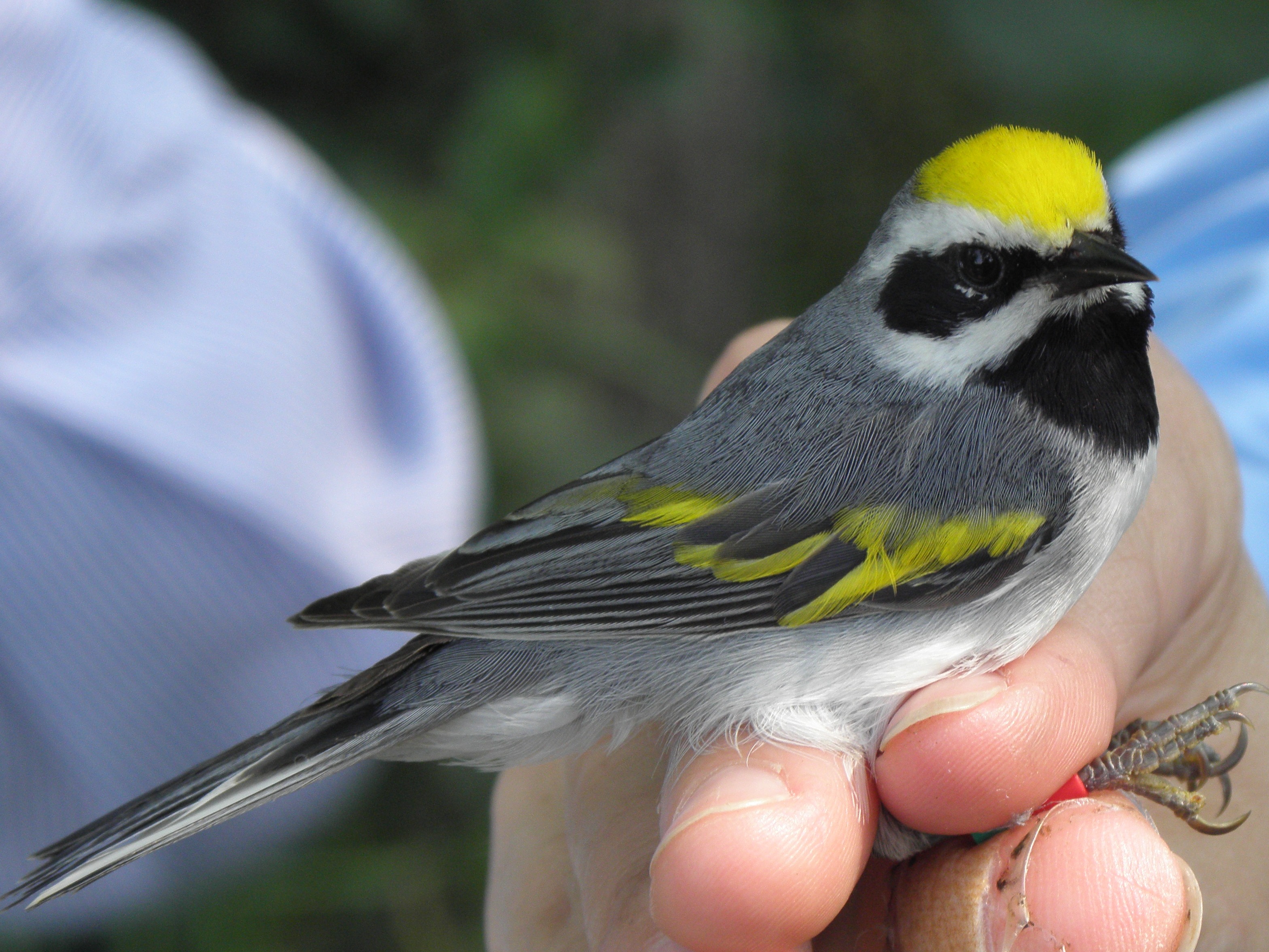
FIGURE 2.4: A golden-winged warbler. Photo: Natural Resources Conservation Service.
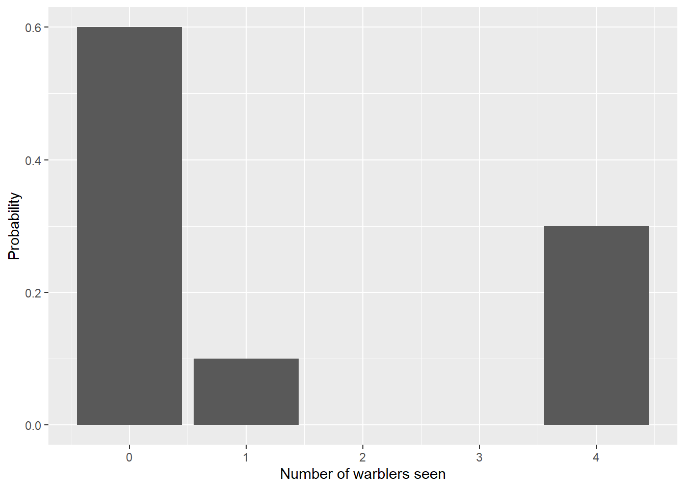
Consider as an example the following probability mass function that a birder has recorded after her research on the golden-winged warbler, a songbird that relies on open areas and patchy woodland habitat for nesting. The researcher noted that it was most likely to see no warblers during a research visit and never saw two or three warblers:
| Number of warblers seen | Probability |
|---|---|
| 0 | 0.6 |
| 1 | 0.1 |
| 4 | 0.3 |
The warbler data can also be represented with the following probability histogram:
We can use the warbler data to find the mean and standard deviation of this discrete random variable. Let \(y\) denote the number of warblers seen and \(\mu\) and \(\sigma^2\) its mean and variance, respectively:
\[\mu = \sum yP(y)\]
\[\mu = (0\times0.6) + (1\times0.1) + (4\times0.3)\]
\[\mu = 1.3\]
So, on average we would expect to see 1.3 warblers given this discrete probability distribution. The variance and standard deviation can also be calculated:
\[\sigma^2 = \sum (y-\mu)^2P(y)\]
\[\sigma^2 = (0-1.3)^2\times(0.6) + (1-1.3)^2\times(0.1) + (4-1.3)^2\times(0.3)\]
\[\sigma^2 = 3.21\]
\[\sigma = \sqrt{\sigma^2} = 1.79\]
So, a typical deviation around the mean is 1.79 warblers, as represented by the standard deviation \(\sigma\).
Consider now if we wish to calculate the sample mean and variance for the number of warblers when we select two samples. To find the sampling distribution of the number of warblers, we could do the following steps:
- list all possible samples than could be observed and their probabilities,
- calculate the mean of each sample,
- list all unique values of the sample mean, and
- sum over all samples to calculate their probabilities.
These steps create a larger number of possibilities. As you can see, even for a sample size of two, we’re beginning to do calculations for a large number of scenarios. The warbler data with two samples can also be seen with the probability histogram:
| Sample 1 | Sample 2 | Probability | Mean |
|---|---|---|---|
| 0 | 0 | 0.36 | 0.0 |
| 0 | 1 | 0.06 | 0.5 |
| 0 | 4 | 0.18 | 2.0 |
| 1 | 0 | 0.06 | 0.5 |
| 1 | 1 | 0.01 | 1.0 |
| 1 | 4 | 0.03 | 2.5 |
| 4 | 0 | 0.18 | 2.0 |
| 4 | 1 | 0.03 | 2.5 |
| 4 | 4 | 0.09 | 4.0 |
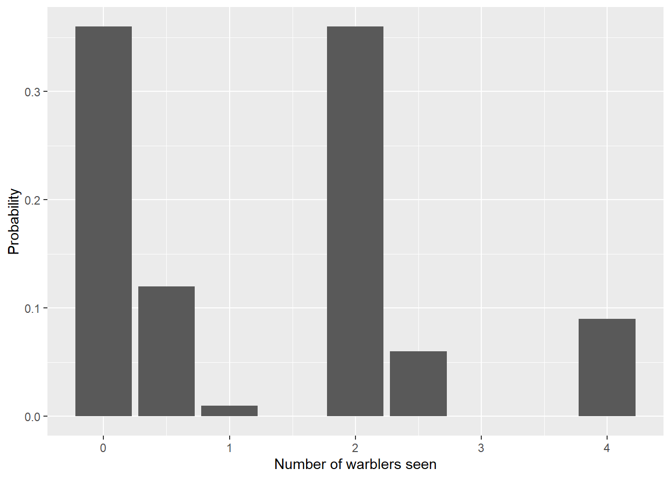
2.3.2 Sampling distribution of the mean
Note the differences between the probability histograms of one and two samples. We will denote the sample mean of collecting two samples as
\[\mu_{\bar{y}} = (0\times0.36) + (0.5\times0.12)+...+(4\times0.09)\]
\[\mu_{\bar{y}} = 1.3\]
So, even after collecting two samples, the mean after collecting two samples is identical to the population mean. The variance and standard deviation of two samples can also be calculated:
\[\sigma^2_{\bar{y}} = \sum (y-\mu)^2P(y)\]
\[\sigma^2_{\bar{y}} = (0-1.3)^2\times(0.36) + (0.5-1.3)^2\times(0.12) + ... + (4-1.3)^2\times(0.09)\]
\[\sigma^2_{\bar{y}} = 1.61\]
\[\sigma_{\bar{y}} = \sqrt{\sigma^2_{\bar{y}}} = \sqrt{1.61}= 1.27\]
Notice the standard deviation of \(\bar{y}\) is smaller than the standard deviation for \(\sigma\). We call the value 1.27 the standard error, defined as the standard deviation of a sampling distribution. The standard error can also be calculated by dividing the standard deviation by the square root of the sample size:
\[\sigma_{\bar{y}} = \frac{\sigma}{\sqrt{n}} \]
\[\sigma_{\bar{y}} = \frac{1.79}{\sqrt{2}} = 1.27 \]
What would happen if we continued to draw more samples of the warbler sightings, say by taking three, five, 10, and 15 samples? No doubt our calculations would become more complex. We are coming up to a big idea in statistics.
2.3.2.1 The central limit theorem
We can continue to take all possible samples of size \(n\) and calculate the sample mean and standard error of the sampling distribution. Using the warbler data, here is the sampling distribution as we increase from three to 15 samples:
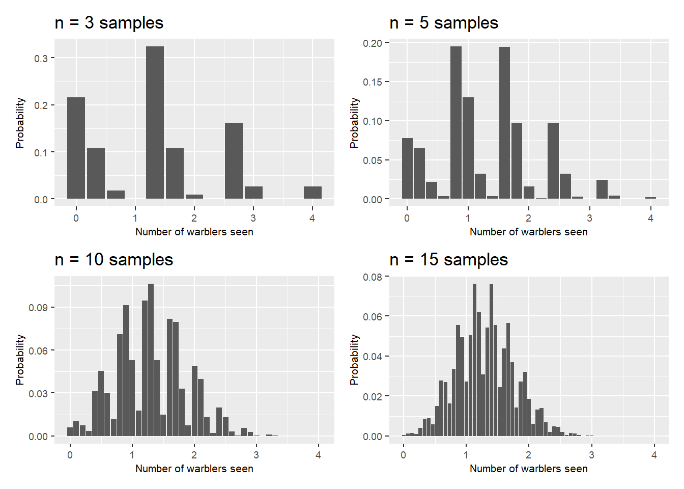
FIGURE 2.5: Visualizing the central limit theorem, from three to 15 samples.
Note that the graphs of the sampling distributions change in appearance as you increase the number of samples. This is the central limit theorem in action. The central limit theorem shows that if you take a large number of samples, the distribution of means will approximate a normal distribution, or a bell-shaped curve. This is a remarkable finding because most population distributions are not normal (i.e., the warbler observations). When a sample is large enough (generally at least 25 observations in the natural resources), the distribution of sample means is very close to normal.
2.3.3 Continuous random variables
A continuous random variable has an “uncountable” number of values where the probability of occurrences move continuously from one value to the next. A continuous random variable Y can be described by a probability density function \(f(y)\), which can be thought of as the area beneath a curve.
For any continuous random variable, the total area beneath the curve must sum to one. Hence, \(P(a < y < b)\) can be considered the area beneath the curve between a and b. Common continuous random variables used in natural resources include the normal, Chi-square, uniform, exponential, and Weibull distributions.
2.3.3.1 Mean and standard deviation of a continuous random variable
When we found the mean and standard deviation for the warbler data, a discrete random variable, we summed across values. However, because continuous random variables have an “uncountable” number of values, the right approach is to integrate across all values to find its mean and standard deviation.
The normal distribution is the foundation for statistical inference throughout this book. The normal distribution describes many kinds of data. Numerous statistical tests assume that data are normally distributed. The mean and standard deviation of a normal distribution are denoted by \(\mu\) and \(\sigma\), respectively.
The mean of a normal distribution is the center of a symmetric bell-shaped curve. Its standard deviation is the distance from the center to specified points on either side. A special case of the normal distribution with a mean of 0 and standard deviation of 1, or N(0,1) is termed the standard normal distribution. Consider, for example, two distributions that have the same mean (\(\mu = 42\)) but different standard deviations (\(\sigma = 3\)) and (\(\sigma = 8\)).
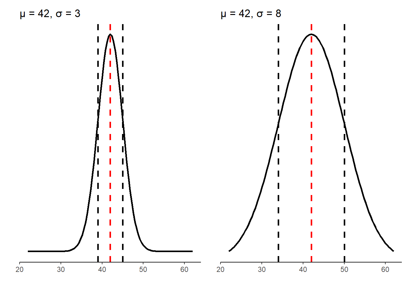
FIGURE 2.6: The normal distribution with the same mean and different standard deviations.
The distributions show that the N(42, 3) distribution is much narrower than the N(42, 8) distribution. This is important because the mean and standard deviation of a normal distribution help define the empirical rule, a rule that describes the approximate percentages of the range of observations. The empirical rule, also referred to as the 68-95-99.7% rule, states that:
- approximately 68% of the observations fall within \(\sigma\) of \(\mu\),
- approximately 95% of the observations fall within \(2\sigma\) of \(\mu\), and
- approximately 99.7% of the observations fall within \(3\sigma\) of \(\mu\).
We can calculate a z-score for any normal distribution. For example, for the N(42, 3) distribution, we can calculate the z-score for the value 38:
\[{z_{38} = \frac {38 - 42}{3}} = -1.33\]
In other words, the value 38 is 1.33 standard deviations less than the mean value of 42. In R, we can write a function called z_score() that calculates a z-score using the three values: the observation of interest \(x_i\), the population mean \(\mu\), and the population standard deviation \(\sigma\):
z_score <- function(x_i, pop_mean, pop_sd){
  z <- (x_i - pop_mean) / pop_sd
  return(z)
}
Then, we can add the values of interest to use the R function to calculate the z-score:
z_score(x_i = 38, pop_mean = 42, pop_sd = 3)## [1] -1.333333So, we know that 38 is 1.33 standard deviations less than the mean.
2.3.4 Exercises
2.7 A deer hunter tells you that there is a 0.7 probability of seeing no deer when he goes hunting, a 0.1 probability of seeing one deer when he goes hunting, and a 0.2 probability of seeing two deer when he goes hunting. Use calculations in R to determine the mean \(\mu\) and standard deviation \(\sigma\) of the number of deer seen from this discrete random variable.
2.8 Mech (2006) published results from a study on the age structure of a population of wolves in the Superior National Forest of northeastern Minnesota, USA. Results indicated a high natural population turnover in wolves.
Looking at Table 1 in the Mech (2006) paper, we can enter the ages and number of wolves in the study using the tribble() function. After creating the data set, plot the wolf age data using a bar plot.
wolves <- tribble(
  ~age, ~num_wolves,
  0, 10,
  1, 9,
  2, 21,
  3, 8,
  4, 9,
  5, 5,
  6, 2,
  7, 2,
  8, 1,
  9, 2
)
2.9 In the wolf data, use calculations in R to determine the mean \(\mu\) and standard deviation \(\sigma\) of the wolf ages.
2.10 Use the z_score() function presented earlier in the chapter to calculate the z-score for a wolf that is six years old.
2.11 Historical data for the amount of lead in drinking water suggests its mean value is \(\mu = 6.3\) parts per billion (ppb) with a standard deviation of \(0.8\) parts per billion. Using concepts from the empirical rule, use R to calculate the upper and lower bounds of the values that are one, two, and three standard deviations away from the mean value.
2.12 An environmental specialist collects data on 15 drinking water samples and calculated a mean lead content of 8.0 ppb. Using the population data in the previous problem, calculate the z-score for this sample.
2.4 Summary
Descriptive statistics are essential components that allow you to better understand the characteristics of your data. Measures of central tendency, spread, and position are values that describe your data and help place it in the context of other observations and data.
By learning about random variables, we have introduced the concepts of probability and how they lead to different outcomes of a chance process. Discrete random variables have a countable number of outcomes whereas continuous random variables have an infinite number of possibilities along a continuous scale. We were introduced to the normal distribution which can be described by a mean and standard deviation and will form the basis of statistical inference. The concepts we learned about the probability as it relates to the normal distribution will be revisited in subsequent chapters when we discuss statistical inference and hypothesis testing.
2.5 References
Freese, F. 1962. Elementary forest sampling. USDA Forest Service Agricultural Handbook No. 232. 91 p.
Gotelli, N.J., and A.M. Ellison. 2002. Biogeography at a regional scale: determinants of ant species density in New England bogs and forests. Ecology 83: 1604–1609.
Mech, L.D. 2006. Estimated age structure of wolves in northeastern Minnesota. Journal of Wildlife Management 70: 1481–1483.
Pierce, G.W. 1943. The songs of insects. Journal of the Franklin Institute 236: 141–146.
Poncet, P. 2019. modeest: mode estimation. R package version 2.4.0. Available at: https://CRAN.R-project.org/package=modeest