Chapter 7 Sample size and statistical power
7.1 Introduction
“Every second of every day, our senses bring in way too much data than we can possibly process in our brains.” This was stated by entrepreneur Peter Diamandis about the role of so-called “big data” in the 21st century. We can spend our entire careers collecting data. (And some people do.) How do we know when we have collected enough data to answer our question of interest? And how confident can we be in the sample we’ve taken to obtain a reliable estimate of the population of interest?
This chapter will provide details for determining the appropriate number of samples to collect. We will revisit concepts from hypothesis testing as it relates to understanding the power of a statistical test.
7.2 How much data should I collect?
In natural resources, data collection costs time, effort, and money. It is rare to have the resources available to measure all of the units in a population, or a complete enumeration. Instead, collecting the appropriate number of samples will help you be efficient with your budget and simultaneously provide reliable data to make decisions. A plan to collect the appropriate number of samples should be designed only after knowing the budget available for the task and the desired precision from our sample to inform what we want to know about the population.
7.2.1 What makes a sample good?
Before we determine how many samples to collect, it is worth discussing what makes a sample good. In natural resources, a good sample has the following characteristics:
- It is unbiased. This means that the sample serves as a useful approximation of the population. Sample bias would result if our expected results differ from the true value being estimated.
- It is efficient. This means that it is easy to obtain the data and the data are representative of the population.
- It is flexible. For example, collecting data on wildlife is challenging because it may mean capturing and releasing live animals. Measuring trees in remote areas can take considerable time and effort to travel to the study site. Flexible samples allow us to address multiple objectives, particularly in cases when the data are difficult to collect.
The goal of sampling is to obtain data that are reliable and will allow you to make inference about a population. A good sample will collect the appropriate number of observations to meet the objectives of the question being asked.
7.2.2 Determining sample size
Determining the appropriate sample size (\(n\)) requires objective and subjective assessments. Objective assessments include determining the variability of the sample, e.g., by calculating its standard deviation. Subjective assessments include specifying the desired confidence level and allowable error of the variable of interest. By having this information prior to the start of a study, a reliable \(n\) can be obtained.
To start, the standard deviation of the variable of interest needs to be obtained to represent its variability. While this may seem challenging because the data have not been collected yet, with minimal effort you can determine the standard deviation using one or more of the following strategies:
- Conduct a pilot study. Consider spending a limited amount of time collecting a few samples to determine the standard deviation for the variable of interest.
- Consult with experts and colleagues. Ask others that may have collected data on your variable of interest and inquire about the variability of their data.
- Research historical data. In natural resources, many species and their populations have been measured and cataloged. Perform a literature review and look for tables and statistical results that report standard deviations for your variable. Consult your organization’s records for historical data that may have been collected on your variable.
- Calculate the standard deviation with a “quick and dirty” approximation. From the empirical rule, we know that nearly all of the data will be found within four standard deviations of the mean (assuming the data are distributed normally). A “quick and dirty” approximation of the standard deviation is \({\sigma} {\approx}{range}/4\). If you have an estimate of the minimum and maximum values for your variable, they can be used to approximate the standard deviation.
Along with the mean, the standard deviation will be used to determine the coefficient of variation (CV) of the variable of interest.
When we talk about confidence, we will also need a value t from the t-distribution to represent the desired confidence interval. To determine the sample size needed at a probability level of 0.90, we can use the qt() function with an infinite number of degrees of freedom (df = Inf), reflecting the large number of observations in the population. We specify the quantile of 0.95 to incorporate 5% of the area on the upper and lower values of the curve:
qt(0.95, df = Inf)## [1] 1.644854So, the t-value for a 90% confidence interval is 1.64.
The final component needed to determine sample size is a subjective assessment of allowable error. The allowable error, represented by A, is expressed as the percent of the mean. For example, A can be set to 10 to estimate the number of samples required to estimate the mean of the population to be within \(\pm10\)%.
The sample size from a simple random sample can be calculated as:
\[n = \Bigg[\frac{(t)(CV)}{A}\Bigg]^2\]
where t, CV, and A represent the t value, coefficient of variation, and allowable error, respectively.

FIGURE 7.1: Yellow perch, a fish native to North America. Photo: US Fish and Wildlife Service.
For example, consider that fisheries biologists want to determine the appropriate number of yellow perch weights to measure. The mean and standard deviation of perch weight is 260 and 101 grams, respectively. If we want to determine the number of samples required to estimate a population mean to within \(\pm10\)% at a probability level of 0.90, we would calculate
\[n = \Bigg[\frac{(1.64)[(101/260)*100]}{10}\Bigg]^2= 40.6\]
After rounding up, we would need to weigh 41 perch to reach the desired precision. In R, the following function num_samples() performs the calculation using the ceiling() function to round up the sample size:
num_samples <- function(t, CV, A){
  n = ((t * CV) / A)**2
  return(ceiling(n))
}

num_samples(t = qt(0.95, df = Inf),
            CV = (101/260)*100,
            A = 10)
## [1] 41You can quickly see that by changing the subjective measures of the calculation (e.g., the t-value associated with the level of confidence), different sample sizes will result. The appropriate number of samples will be based on your desired level of precision and available resources to collect the data. (A series of upcoming exercises will investigate how changing the coefficient of variation and the allowable error A results in different sample sizes.)
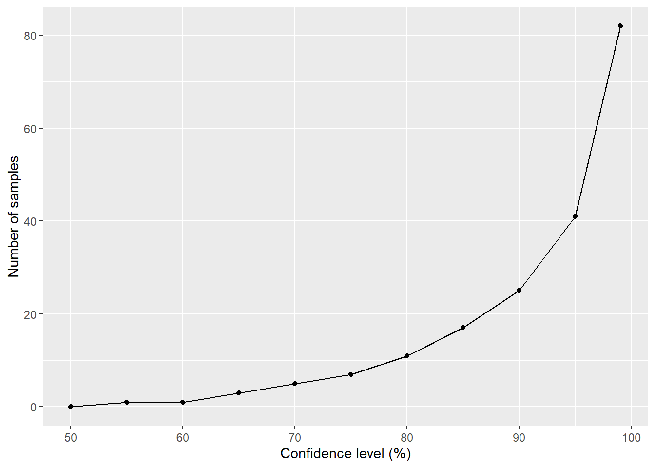
FIGURE 7.2: Changes in the number of samples of yellow perch weights needed to maintain a desired level of precision with an allowable error of 10%.
7.2.3 Exercises
7.1 Write a function that calculates a “quick and dirty” approximation of the standard deviation as mentioned in this chapter, where \({\sigma} {\approx}{range}/4\). Use it to calculate approximate standard deviations for the following variables:
- A population of perch weights with a maximum and minimum of 350 and 60 grams, respectively.
- The ages of white-tailed deer of 2, 3, 3, 4, 6 and 7 years.
- The height (
HT) of cedar elm trees (in feet) from the elm data set.
7.2 Consider a quantitative variable that interests you (e.g., the weights of perch; the heights of cedar elm trees). Perform an internet search to find a scientific article or publication that reports a mean and standard deviation for this value. Use R code to calculate the coefficient of variation for this variable of interest.

FIGURE 7.3: Strawberries. Image: domdomegg/Wikimedia Commons.
7.3 A strawberry farmer collects some data on yields from different fields on her farm. She collects data from five fields and records yields of 48,000, 52,000, 65,000, 58,000, and 56,000 pounds per acre. Use the num_samples() function to determine the appropriate number of samples to collect under the following scenarios.
- Find the sample size necessary to estimate a population mean with 95% confidence with an allowable error of 5%.
- Find the sample size necessary to estimate a population mean with 99% confidence with an allowable error of 5%.
7.4 Foresters measure the diameters of logs to sell to a sawmill. Data are a sample from a population of hundreds of logs from a recent timber harvest. They calculate a mean log diameter of 22.6 inches and a standard deviation of 8.5 inches. Use the num_samples() function to determine the appropriate number of samples under the following scenarios.
- Find the sample size necessary to estimate a population mean with 90% confidence with an allowable error of 15%.
- How many more logs need to be sampled if the coefficient of variation of the logs is doubled?
- How many fewer logs need to be sampled if the coefficient of variation of the logs is cut in half?
- How many fewer logs need to be sampled if the allowable error of the logs is doubled?
- How many more logs need to be sampled if the allowable error of the logs is cut in half?
7.3 Statistical power
We learned in Chapter 4 that Type II error occurs when we fail to reject the null hypothesis when it is in fact false, denoted by \(\beta\). The probability of correctly rejecting the null hypothesis when it is indeed false is \(1-\beta\), also known as the statistical power of a hypothesis test.
7.3.1 Defining statistical power
To understand statistical power, it is worth revisiting the concepts of p-values. A p-value is the probability under a specified statistical model that a statistical summary of the data would be equal to or more extreme than its observed value. If the p-value is smaller than some pre-defined significance level termed \(\alpha\) (typically set to 0.05), the result is said to be statistically significant.
The probability of obtaining a statistically significant result is called the statistical power of the test. The power of a test relies on the size of the effect and the sample size.
Statistical power ranges from 0 to 1. As power increases, the probability of making a Type II error decreases. In natural resource sciences, specifying a statistical power of 0.80 is common.
7.3.2 Calculating the power of statistical tests
R’s power.t.test() function determines the power of a statistical hypothesis test. You will need to know several things prior to calculating the power:
- the null and alternative hypotheses for your test,
- whether you’re conducting a one- or a two-sided test, paired test, or test of proportions,
- the sample size,
- the sample mean and standard deviation,
- the difference between your hypothesized mean value and your sample mean (represented by
delta =), and - the significance level \(\alpha\).
For example, we can calculate the power of a two-sided one-sample t-test on the weights of yellow perch. Consider a sample of 150 perch with \(\bar{y} = 260\) and \(s = 101\) grams. The null hypothesis \(H_0\) is that the true mean is equal to 240 grams and the alternative hypothesis \(H_1\) is that the true mean is not equal to 240 grams:
power.t.test(n = 150,
             delta = 260 - 240,
             sd = 101,
             sig.level = 0.05,
             type = "one.sample",
             alternative = "two.sided")
##
## One-sample t test power calculation
##
## n = 150
## delta = 20
## sd = 101
## sig.level = 0.05
## power = 0.6735067
## alternative = two.sidedNote the output provides you the power of the t-test. A greater power indicates that we have a much better ability to detect a difference if one exists. The results from this test indicate we have a 67% chance of finding a difference if one exists in the population.
We can also use the power.t.test() function to perform a two-sample t-test on the weights of yellow perch. Consider two samples of perch with 150 observations each with \(\bar{y_1} = 240\) \(\bar{y_2} = 270\). The null hypothesis \(H_0\) is that the two means are equal and the alternative hypothesis \(H_1\) is that the true means are not equal:
power.t.test(n = 150,
             delta = 240 - 270,
             sd = 101,
             sig.level = 0.05,
             type = "two.sample",
             alternative = "two.sided")
##
## Two-sample t test power calculation
##
## n = 150
## delta = 30
## sd = 101
## sig.level = 0.05
## power = 0.7271084
## alternative = two.sided
##
## NOTE: n is number in *each* groupThe results from this two-sample test indicate we have a 73% chance of finding a difference if one exists in the population. You may change the argument to alternative = "one.sided" to find the power of a one-sided test.
The power.t.test() function can also be used for calculating the power of a paired t-test by changing type = "paired". For proportions, the power.prop.test() function can calculate the power of two-sample tests.
We can also use the power.t.test() function to ask how many samples are needed to achieve a desired level of power. If we state n = NULL in the code and specify power = 0.80, the function will tell us how many samples would be needed to achieve 0.80 power.
Using the two-sided one-sample t-tests on yellow perch weights described above, the following code will find the number of samples needed to carry out a two-sided one-sample t-test with 99% confidence. The null hypothesis is that yellow perch weight is equal to 240 grams and an alternative hypothesis that weight is not equal to 240 grams:
power.t.test(n = NULL,
             delta = 260 - 240,
             sd = 101,
             power = 0.80,
             sig.level = 0.01,
             type = "one.sample",
             alternative = "two.sided")
##
## One-sample t test power calculation
##
## n = 301.1659
## delta = 20
## sd = 101
## sig.level = 0.01
## power = 0.8
## alternative = two.sidedWe would need to collect 301.1659, or 302 samples of yellow perch weight to achieve the desired power of 0.80.
We can perform a similar calculation on proportions with the power.prop.test() function. For example, consider two technicians that inspect facilities for hazardous waste compliance. There is a probability of 0.21 and 0.32 that they will issue a violation on each visit. A 0.75 power calculation with a significance level \(\alpha = 0.05\) would be:
power.prop.test(n = NULL,
                power = 0.75,
                p1 = 0.21,
                p2 = 0.32,
                sig.level = 0.05)
##
## Two-sample comparison of proportions power calculation
##
## n = 222.548
## p1 = 0.21
## p2 = 0.32
## sig.level = 0.05
## power = 0.75
## alternative = two.sided
##
## NOTE: n is number in *each* groupWe would need to collect 222.548, or 223 samples from each technician to achieve the desired power of 0.75.
7.3.3 Exercises
7.5 For the following questions, use the elm data set and conduct the analyses with a significance level of \(\alpha = 0.10\).
- Calculate the power of a two-sided one-sample t-test on the height (
HT) of elm trees. The null hypothesis of the test is that the true mean of all trees is equal to 30 feet and the alternative hypothesis that the true mean is not equal to 30 feet. - Calculate the power of a two-sided one-sample t-test on the height (
HT) of all co-dominant elm trees. The null hypothesis of the test is that the true mean of co-dominant elm trees is equal to 34 feet and the alternative hypothesis that the true mean is not equal to 34 feet. - Find the number of samples of elm trees needed to achieve 0.85 power based on the hypothesis test outlined in part a.
- Find the number of samples of co-dominant elm trees needed to achieve 0.70 power based on the hypothesis test outlined in part b.
7.6 Using the hypothesis test in question 7.5a, find the number of samples of elm trees needed to achieve different levels of power ranging in ten percent increments from 0.50 to 0.90. Make a plot using ggplot() that shows the influence of power on the sample size.
7.7 The following proportions of ruffed grouse showed antibodies consistent with West Nile virus in different US states: Michigan (0.13), Minnesota (0.12), and Wisconsin (0.29). Calculate the number of grouse samples needed in each state to achieve a power of 0.80 at a significance level \(\alpha = 0.05\) using the following two-sided tests:
- Michigan and Minnesota
- Michigan and Wisconsin
- Minnesota and Wisconsin
- Why do the sample sizes required in the previous tests differ?
7.4 Summary
Determining the appropriate number of samples to collect is a critical part of natural resources science and management. Sampling efforts in natural resources need to be unbiased, flexible, and efficient. Understanding our variables of interest before collecting a thorough sample will assist us by knowing the variability we should expect in the population. All efforts that determine sample size rely on both objective (e.g., standard deviation) and subjective (e.g., significance level) assessments.
When combined with a planned hypothesis test, the power of a statistical test allows us to minimize Type II error, or failing to reject the null hypothesis when it is in fact false. Tests of power can be conducted with the familiar hypothesis tests we learned in Chapter 4, including one- and two-sample and paired t-tests. A thorough understanding of the statistical concepts of sample size and power allows you to design an efficient sampling scheme, saving you time and energy by not oversampling.