Chapter 3 Probability
3.1 Introduction
Probability is so widespread in statistics that we’ve already talked about it in depth in the first two chapters. Probability is based on randomness, the process by which outcomes are uncertain with some distribution. We may or may not know what the distribution of outcomes is, but can find it after a large number of repetitions. By understanding randomness and probability, we will ease into the discipline of statistical inference, where we will talk about hypothesis testing and estimation.
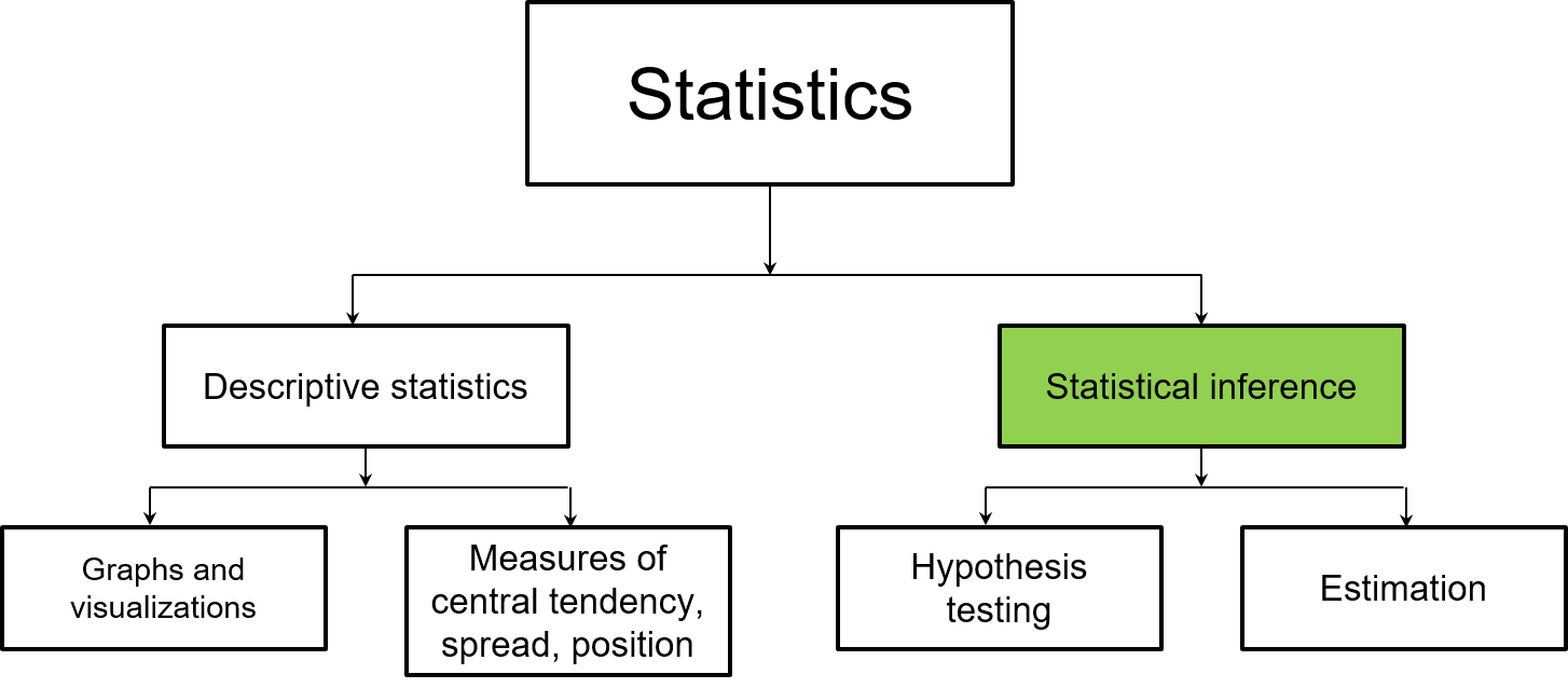
FIGURE 3.1: This chapter focuses on probability, and introduces topics related to statistical inference.
Consider a tree that is subject to infestation by a non-native insect that can lead to its death. The concepts of probability are based on several definitions:
- A random experiment is any observation or measurement that has an uncertain outcome. For example, a forest health specialist may conduct an assessment of the tree to determine whether or not the insect is present (i.e., the tree shows symptoms of the insect damage) or absent (the tree is healthy).
- A sample space is a list of all possible outcomes of an experiment. For example, the insect is present on the tree or not.
- An event is any collection of one or more outcomes from an experiment. For example, the forest health specialist visits one tree or one hundred trees and records whether or not the insect is present.
- The probability of any outcome is the proportion of times an event would occur over repeated observations.
Probability allows us to use information from populations to inform samples. Statistical inference allows us to generalize from samples to make statements about populations. Together, these relationships will serve as the foundation for much of the rest of this book.

FIGURE 3.2: Probability allows us to use information from populations to inform samples.
Note the differences between the statements below with regard to probability versus statistical inference. Are they the same?
A probability approach: A forest health specialist manages 100 ash trees in a city. Fifteen of these trees show symptoms of emerald ash borer, a invasive insect that leads to ash tree mortality in North America. The forest health specialist samples 10 of these ash trees. What is the chance that three of the ten trees show symptoms of emerald ash borer?
A statistical inference approach: Ten ash trees are sampled in a metropolitan area with 1000 ash trees. Three ash trees show symptoms of emerald ash borer. What is the proportion of ash trees that have emerald ash borer?
This chapter will discuss how the concepts of probability can be used in R to better understand natural resources data. This will allow us to make inferences that will aid us in making statements about data.
3.2 The five rules of probability
The following rules introduce guidelines for probability. These will assist us when performing calculations and creating visualizations of events.
3.2.1 Rule 1: Probabilities are between 0 and 1
Any probability is a value between 0 and 1. Values range from 0 (impossible) to 1 (certain). You may often hear about probabilities discussed in terms of percentages, likelihoods, or odds. The key when using probabilities in calculations is that they are always expressed in decimal form, and not percentages. For example, there is a 0.60 probability of having a drought this year, not a 60% chance of having a drought.
Understanding a probability value is important, but where do probabilities come from? If we know how many outcomes to expect, this is an example of using a classical approach to assign probabilities. If an experiment has \(n\) outcomes, we can assign a probability of \(1/n\) to each outcome. For example, what is the probability we flip a coin and get a head?
We could also rely on past experiments or trends to assign probabilities. In this example, probabilities are derived from historical data or experiments. Due to the experimental nature of this approach, it is important to note that different experiments will typically result in different probabilities. For example, if you flip a coin ten times you might get a head four times. If you repeat the experiment, you might get a head seven times. In other words, if \(n_A\) is the number of times that event \(A\) occurred, \(n_A/n\) represents the frequency at which \(A\) occurs.
A third way to assign probabilities is using a subjective approach. In this approach, the probability is based on intuition or prior knowledge. While subjective approaches may be useful, they are not always based on data or can make important assumptions about the variables of interest. For example, a researcher might say there is a 0.60 probability of having a drought this year based on her “gut instinct.”
DATA ANALYSIS TIP: Many disciplines, such as sports and weather forecasting, use a mix of approaches to determine probabilities. The Old Farmer’s Almanac, a reference book for weather forecasts in the United States, indicates an average accuracy rate of 80% for its annual weather predictions. This rate is calculated by comparing their predicted changes in temperature and precipitation to the actual observed changes in different areas of the US (The Old Farmer’s Almanac 2020). Note that these accuracy numbers are self-reported.
3.2.2 Rule 2: All probabilities sum to one
To determine if a probability model is appropriate, sum up all of the probabilities. Their sum should add to one. In other words, all probabilities of events in the sample space should add to one. Venn diagrams are useful to see how the events are related, such as the probability of events A and B occurring. A Venn diagram will show if two events are mutually exclusive, i.e., if two events can occur with one repetition of an experiment.
Consider the following example of common North American tree species and their clade (angiosperm or gymnosperm) and whether or not they are deciduous (i.e., their leaves fall after the growing season):
| Common name | Scientific name | Clade | Deciduous |
|---|---|---|---|
| Sugar maple | Acer saccharum | Angiosperm | Yes |
| Yellow poplar | Liriodendron tulipifera | Angiosperm | Yes |
| White oak | Quercus alba | Angiosperm | Yes |
| Red maple | Acer rubrum | Angiosperm | Yes |
| Northern red oak | Quercus rubra | Angiosperm | Yes |
| Douglas-fir | Pseudotsuga menziesii | Gymnosperm | No |
| Loblolly pine | Pinus taeda | Gymnosperm | No |
| Ponderosa pine | Pinus ponderosa | Gymnosperm | No |
| Lodgepole pine | Pinus contorta | Gymnosperm | No |
| Western hemlock | Tsuga heterophylla | Gymnosperm | No |
| Tamarack | Larix laricina | Gymnosperm | Yes |
| Bald cypress | Taxodium distichum | Gymnosperm | Yes |
We can say that the clade of a tree is mutually exclusive (or “disjoint”) because a tree can only be a gymnosperm or angiosperm:
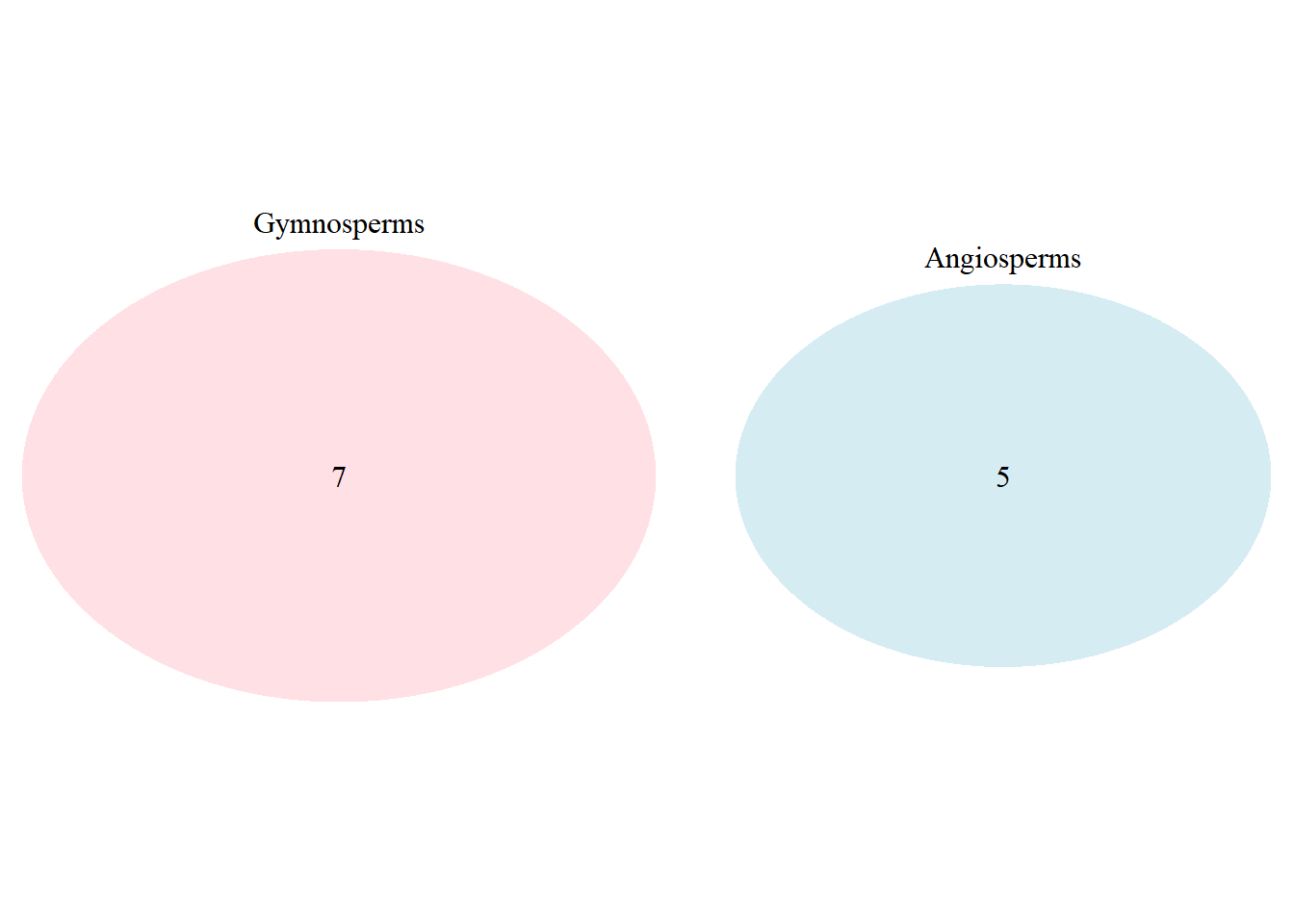
FIGURE 3.3: Venn diagram showing the clades of trees, events that are mutually exclusive.
Venn diagrams will be useful to create and examine to make sure your model follows the rules of probability.
3.2.3 Rule 3: If two events are mutually exclusive, apply the addition rule
If two events do not share the same outcomes and are mutually exclusive, the probability that one or the other occurs is the sum of their individual probabilities. This is termed the addition rule of probability. This can be written as:
\[P(A \bigcup B)=P(A)+P(B)\]
The notation \(P(A \bigcup B)\) can be thought of as the probability of A or B occurring. Take for example the tree data set with 10 different species. We can determine the probability of selecting a tree from the maple (Acer) or pine genus (Pinus). We know that \(P(maple)=2/10\) and \(P(pine)=3/10\). We can then write
\[P({\mbox{maple }} \bigcup {\mbox{ pine}})=2/12+3/12 = 0.4167\]
Maples and pines are common in the data set and there is about a 42% chance we would select one of those species at random.
3.2.4 Rule 4: The complement of a probability is measured when it does not occur
The complement of any event A is the probability that A does not occur, defined as \(P(A^C)\). In other words, if the probability of choosing a maple tree from our data set is 2/12 = 0.1667, the probability of not choosing a maple tree is 10/12 = 0.8333. More generally, the complement of a probability can be written as \(P(A^C) = 1 - P(A)\).
The idea of the complement of a probability is highlighted with a well-known observation in probability known as the birthday problem (Feller 1968). Suppose there are n people in a room at one time. What is the probability that two people in that room share the same birthday? Rather than finding the probability of an event, it’s often easier to find the probability of it not occurring (i.e., the complement).
To determine the probability of a birthday match, we’ll make a few assumptions:
- Birthdays are independent of one another. That is, there are no twins in the room.
- Birthdays are distributed evenly across the year.
- We’ll consider only non-leap years with 365 days in the year.
Then we can say that the probability of two students not sharing the same birthday is 364/365. If there are n people in the room, we can state that
\[P({\mbox{at least one birthday match}})=1-(\frac{364}{365}\times\frac{363}{365}\times ...\times\frac{365-n}{365})\]
It turns out that if there are 23 people in a room, there is about an even chance that at least two people in the room will share the same birthday. These somewhat surprising results are a reflection that there are so many possible pairs of birthdays. As the number of people in a room increases, the probabability of a birthday match increases.
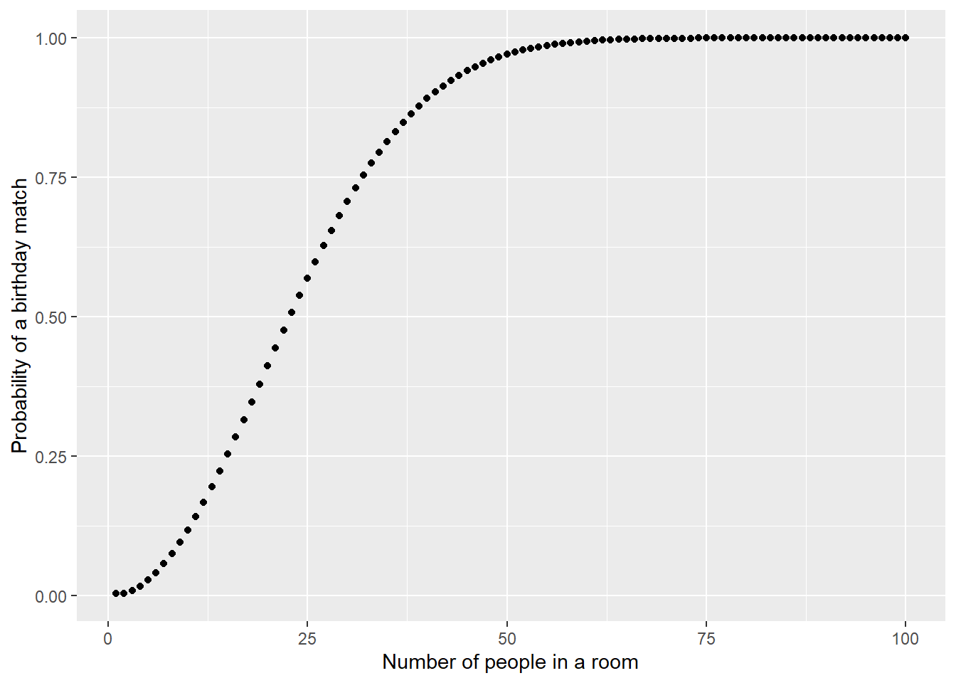
FIGURE 3.4: Probability of a birthday match with different number of people in a room.
While it may be difficult to find the probability of an event, the birthday problem shows us that calculating the complement of an event is often easier.
3.2.5 Rule 5: If one event happening does not influence another, the events are independent
Two events are independent if knowing that one event occurs does not change the probability that the other occurs. In other words, if two events \(A\) and \(B\) do not influence each other, and if knowledge about one does not change the probability of the other, the events are independent.
The probability we assign to an event can change if we know that some other event has occurred. This is common in natural resources because we often collect data across time (e.g., weather patterns today can influence how plants grow tomorrow) and space (e.g., plants will not have the same growth rate if grown at different densities with varying levels of light and nutrients). When we calculate the probability that one event will happen given that another event has occurred, we are determining a conditional probability. The conditional probability of event \(A\) occurring given event \(B\) has already occurred can be written as:
\[P(A|B)=\frac{P(A {\mbox{ and }} B)}{P(B)}\] We can interpret the pipe “|” by saying “given” or “conditioned on.” Whether or not events are independent can inform how to calculate probabilities. You can use conditional probability to assess if two events are independent. If \(P(A|B)=P(A)\) or \(P(B|A)=P(B)\), the events are independent. Otherwise, the events are dependent and additional considerations are required to determine their associated probabilities.
3.2.6 Exercises
3.1 A single tree species is sampled randomly from the table of 12 common trees in North America shown earlier in this chapter. Find the probability of the following:
- A tree is an angiosperm.
- A tree is from the Quercus (oak) genus.
- A tree is not deciduous.
3.2 Now, assume that three tree species are sampled randomly (without replacement) from the table of 12 common trees in North America shown earlier in this chapter. Find the probability of the following:
- Three trees are sampled from the Pinus (pine) genus.
- Three trees sampled are gymnosperms.
- The first two trees sampled are gymnosperms and the last species is an angiosperm.
- Three trees sampled are angiosperms or three trees are sampled from the Pinus (pine) genus.
3.3 In a forest, 30% of the trees suffered damage from an insect and were affected by a disease. A total of 65% of those trees only suffered damage from an insect. What is the probability of a tree being affected by a disease given it already suffered damage from an insect?
3.4 Use the following function, birthday(), in R to calculate the probability of two people sharing the same birthday if 5, 20, and 40 people are in a room together (i.e., n = 5, 20, and 40). Note that q calculates each of the probabilities of not sharing the same birthday and p sums those probabilities. The probability is printed in the output.
birthday <- function(n){
  q <- 1 - (1:(n - 1)) / 365
  print(p <- 1 - prod(q))
}
3.5 By memory, list the birthdays and names for all of your close friends and family members. List any number of birthdays that come to memory. Use the birthday() function in the above problem to determine the probability of two of them sharing the same birthday. Do any of your close friends and family members share the same birthday?
BAYES’ THEOREM: If prior knowledge related to an event is known, Bayes’ Theorem can be used to determine the probability of an event. The probability of event A occurring given that B is true can be determined with the formula below. Bayes’ Theorum is used so widely that it led to the creation of a discipline within statistics termed Bayesian statistics. More generally, the conditional probability P(B|A) represents the likelihood of the event occurring, i.e., the degree to which event B is supported by event A. The prior probability is represented by P(A), representing a subjective or objective belief about the probability before data are considered. The data themselves, also known as the “evidence,” are represented by P(B). The conditional probability P(A|B) of interest is referred to as the posterior probability with Bayesian statistics.
\[P(A|B) = \frac{P(B|A)P(A)}{P(B)}\]
3.3 Probability functions in R
In R, we can use the sample() function to randomly sample from a list. This function will be helpful in many aspects of probability. For example, we can sample two random species from the tree data set:
sample(tree$`Common name`, 2)## [1] "Lodgepole pine" "White oak"By default, the sample() function will select from a list without replacement. We can add to the code to select two trees with replacement.
sample(tree$`Common name`, 2, replace = TRUE)## [1] "Douglas-fir" "Douglas-fir"The prod() function multiplies several values together. This can be useful to when sampling without replacement, as the number of remaining samples will decrease by one after each iteration. For example, consider that we want to sample two species from the tree data set containing 12 species. We could find the probability of selecting two specific species as:
(1/12) * (1/11) ## [1] 0.007575758Or with the prod() function we could write
1 / prod(12:11)## [1] 0.007575758where a colon : indicates a sequence of values to multiply, i.e., “from 12 to 11.” The sum() function works similarly and will add a sequence of numbers together. The cumprod() and cumsum() functions provide the cumulative product and sum of a sequence of values.
When calculating probabilities in R, the choose() function calculates the total number of possibilities of a subset of events occurring. In our example using the tree data set, we can find the total number of possibilities for selecting two unique species from the larger list of 12 species:
choose(12, 2)## [1] 66There are 66 total possibilities for selecting two unique species from the list of 12 species. The choose() function represents a combination of outcomes and can be written as \(n \choose k\), where \(n\) items are sampled \(k\) times without replacement. It can be calculated using factorials, i.e.,
\[{n \choose k} = \frac{n!}{k!(n-k)!}\]
In the tree data set, \(12!\) (pronounced “12 factorial”) equates to \(12 * 11 * 10 * ... * 1\). Hence,
\[\frac{12!}{2!(12-2)!}\]
results in the 66 total possibilities.
3.3.1 Exercises
3.6 A plant ecologist wants to randomly sample 5 plants from a total of 20 plants (numbered 1 through 20) to determine the presence of a foliage disease. Use the sample() function in R to determine which plants to sample without replacement.
3.7 Now, use the sample() function in R to sample 5 plants with replacement.
3.8 Use the choose() function to calculate the total number of possibilities of selecting four unique plants to measure from the 20 total plants.
3.9 Use the choose() function to calculate the probability of sampling (without replacement) the following four plant numbers: 6, 14, 15, and 19.
3.10 Instead of the choose() function, use the formula for the combination of outcomes to arrive at the same answer as in 3.9 but only by using the prod() function.
3.4 Discrete probabilities: the Bernoulli and binomial distributions
The Bernoulli and binomial distributions are two examples of discrete distributions. Understanding them can help to interpret probabilities. The Bernoulli distribution is a discrete distribution having two possible outcomes: success or failure. A binomial distribution is a sum of Bernoulli trials. When the same chance process is repeated several times, we are often interested in whether a particular outcome does or does not happen on each repetition. In some cases, the number of repeated trials is fixed in advance, and we are interested in the number of times a particular event occurs.
Flipping a coin and observing whether it is heads or tails is an example of a Bernoulli trial. With a fair coin, the probability of getting a heads is p = 0.5. The Bernoulli distribution is the simplest discrete distribution, and is the foundation for other more complicated discrete distributions.
In mathematical terms, \({\mbox{Binomial = Bernoulli + Bernoulli + ... + Bernoulli}}\). The binomial distribution is measured by the count of successes (X) with parameters n and p, where:
n is the number of trials of the chance process,
p is the probability of a success on any one trial, and
the possible values of X are the whole numbers from 0 to n.
If a count has a binomial distribution with n trials and probability of success p, the mean can be determined as np and the standard deviation as np(1-p).
The formula for finding the probability of exactly x successes is:
\[{P(X=x)}=\frac{n!}{x!(n-x)!}{p^x}{(1-p)}^{n-x}\]
The binomial distribution requires knowledge of the combination of outcomes to determine the probability of x successes.
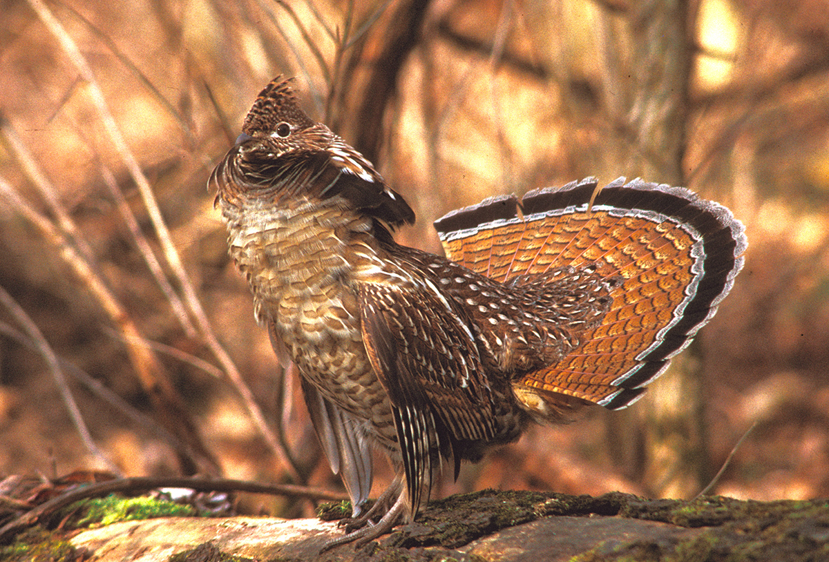
FIGURE 3.5: Ruffed grouse, a North American forest bird. Image: Ruffed Grouse Society.
As an example application of the binomial distribution, consider the relationship between ruffed grouse (Bonasa umbellus) and West Nile virus (from the genus Flavivirus). Wildlife biologists are interested in knowing how the virus, a mosquito-borne disease, impacts the health of ruffed grouse, a forest bird located across North America and a popular game species. Researchers have hypothesized that the introduction of West Nile virus in the early 2000s in North America has led to population declines in ruffed grouse (Stauffer et al. 2017).
In 2018, a multi-state effort examined the presence of West Nile virus in ruffed grouse populations across the US Lake States. The study concluded that while the West Nile virus was present in the region, grouse that were exposed to West Nile did not always die and many survived. The total number of ruffed grouse sampled in each of the three states, and those that showed antibodies consistent with West Nile virus is shown in the table below:
| State | Number of grouse sampled | Number of grouse with West Nile | Proportion of grouse with West Nile |
|---|---|---|---|
| Michigan | 213 | 28 | 0.13 |
| Minnesota | 273 | 34 | 0.12 |
| Wisconsin | 235 | 68 | 0.29 |
Using the grouse data, we can think of whether or not a grouse has West Nile as a Bernoulli trial. If a group of grouse are sampled, some number of them may have the West Nile virus, and we have a binomial distribution.
As an example, consider a random sample of six grouse from Michigan. What is the probability that none of these grouse will have the West Nile virus? The problem can be solved with the binomial formula assuming \(x = 0\) grouse are infected with West Nile from a total of \(n = 6\) grouse. The probability of a grouse having West Nile virus in Michigan is \(p = 0.13\):
\[{P(X=0)}=\frac{6!}{0!(6-0)!}{0.13^0}{(1-0.13)}^{6-0}=0.4336\]
Or, there would be about a 43% chance that if you sampled six grouse from Michigan, none of them would have the West Nile virus.
Below shows a function p.binomial() that creates “pin probabilities” showing the results of a binomial problem. The visualization shows a sample of \(n = 6\) ruffed grouse from Michigan and calculates the probability of each possible number of grouse being infected with West Nile. Note the ymax and xmax statements specify the length of the y and x axes, respectively:
p.binomial <- function(n, p, title, ymax, xmax){
  x <- dbinom(0:n, size = n, prob = p)
  barplot(x, ylim = c(0, ymax), xlim = c(0, xmax),
          names.arg = 0:n,
          xlab = "Number of grouse with West Nile",
          ylab = "Probability",
         main = sprintf(paste(title)))
}

p.binomial(6, 0.13,
           "Binomial distribution (n = 6, p = 0.13)",
           0.5, 7)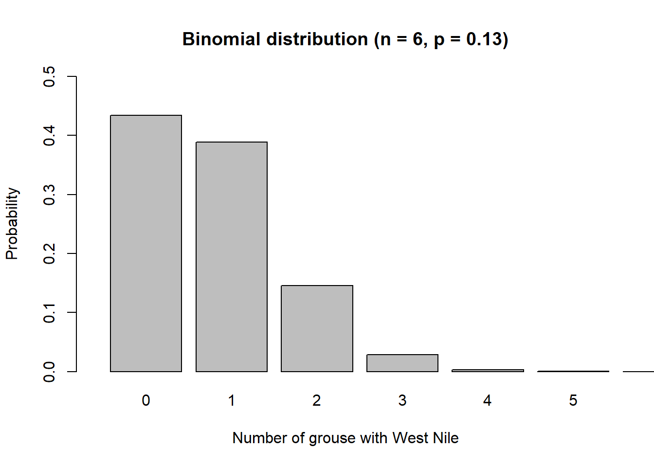
We can see that if six grouse are sampled in Michigan, the most probable outcome is that zero ruffed grouse will have West Nile. We can modify the function to visualize how many grouse in Wisconsin may be infected with West Nile virus if a sample of \(n = 50\) are taken:
p.binomial(50, 0.29, "Binomial distribution (n = 50, p = 0.29)",
           0.15, 51)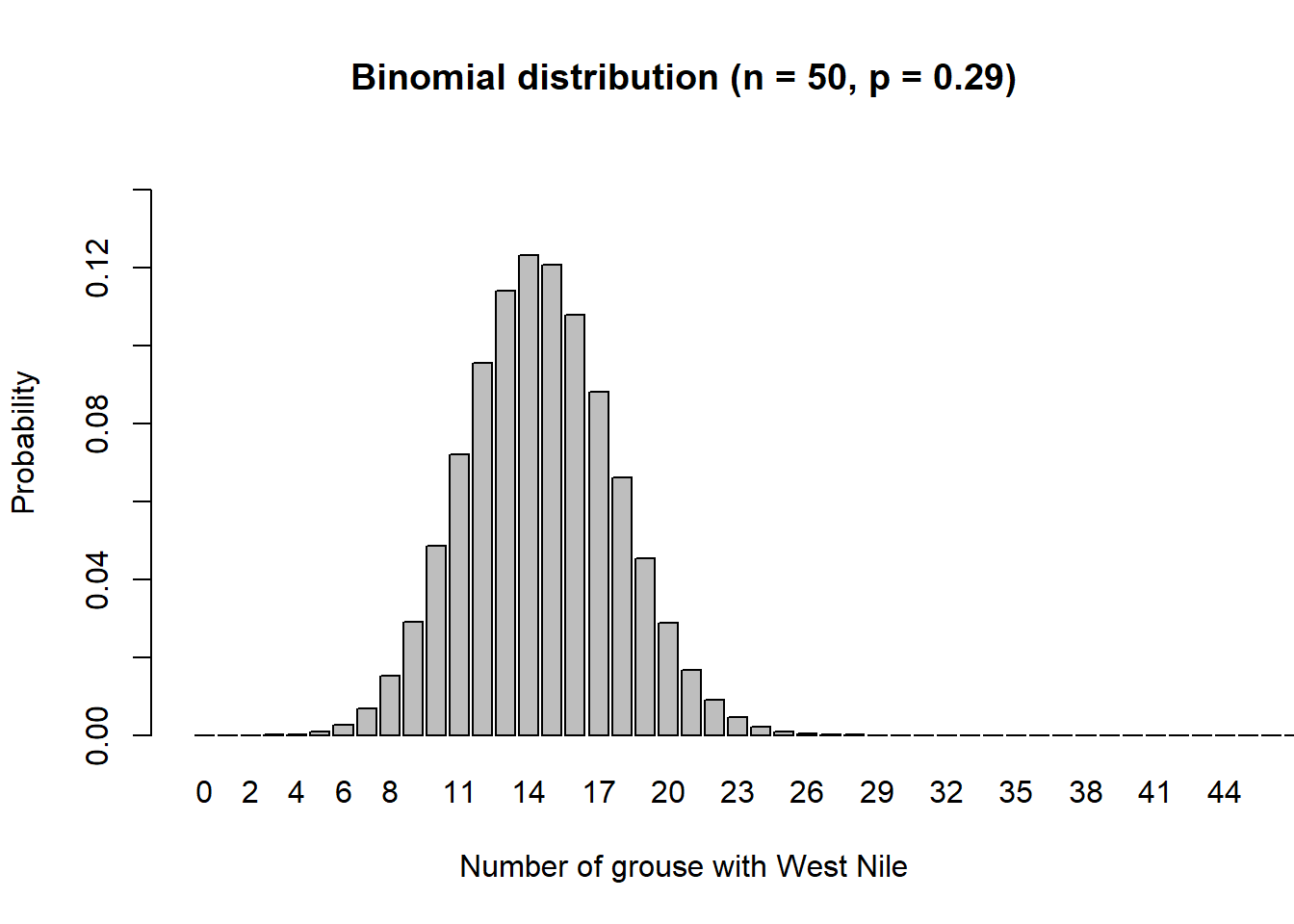
We can see that if 50 grouse are sampled in Wisconsin, the most probable outcome is that between 12 and 16 ruffed grouse will have West Nile.
One of the key characteristics of a discrete distribution is that values may only take on distinct values. In R, several density functions allow for calculating probabilities of events from specific distributions. The dbinom() function provides the density for a binomial distribution with parameters x, size, and prob. We can use the dbinom() function to find the probability that no grouse from a random sample of six grouse in Michigan will have the West Nile virus:
dbinom(x = 0, size = 6, prob = 0.13) ## [1] 0.4336262We might be interested to know the probability of 0 or 1 or 2 grouse being infected with West Nile from a random sample of six grouse in Michigan. In this case, we can add a series of binomial densities together to determine the probability:
dbinom(x = 0, size = 6, prob = 0.13) +
  dbinom(x = 1, size = 6, prob = 0.13) +
  dbinom(x = 2, size = 6, prob = 0.13)
## [1] 0.9676241Alternatively, the pbinom() function provides the distribution function of the binomial. Probabilities are summed up to and including the value specified in the q parameter:
pbinom(q = 2, size = 6, prob = 0.13) ## [1] 0.9676241While the binomial distribution is common in natural resources, other discrete random variables include the geometric, Poisson, and negative binomial.
3.4.1 Exercises
3.11 Consider a random sample of 25 grouse. Use the table that shows the state results of West Nile occurrence and the binomial functions to calculate the following probabilities.
- Use the
p.binomial()function to make a plot of the probabilities of grouse in Minnesota being infected with West Nile virus. - What is the probability that five grouse from Minnesota will have the virus?
- What is the probability that five or fewer grouse from Minnesota will have the virus?
- What is the probability that six or more grouse from Minnesota will have the virus?
3.12 You are tasked with inspecting the facilities of companies that store hazardous waste as a part of their operations. If the company is not storing the waste safely (e.g., the material is not labeled properly or it is improperly stored), you will issue the company a violation. You inspect eight facilities for hazardous waste compliance and you know from historical records that there is a probability of 0.24 they will be issued a violation.
- Modify the
p.binomial()code to make a plot of the probabilities of issuing violations. - Use R code to calculate the mean and standard deviation of violations for this binomial distribution.
- What is the probability that two facilities will be issued a violation?
- What is the probability that two or fewer facilities will be issued a violation?
3.5 Continuous probabilities: the normal distribution
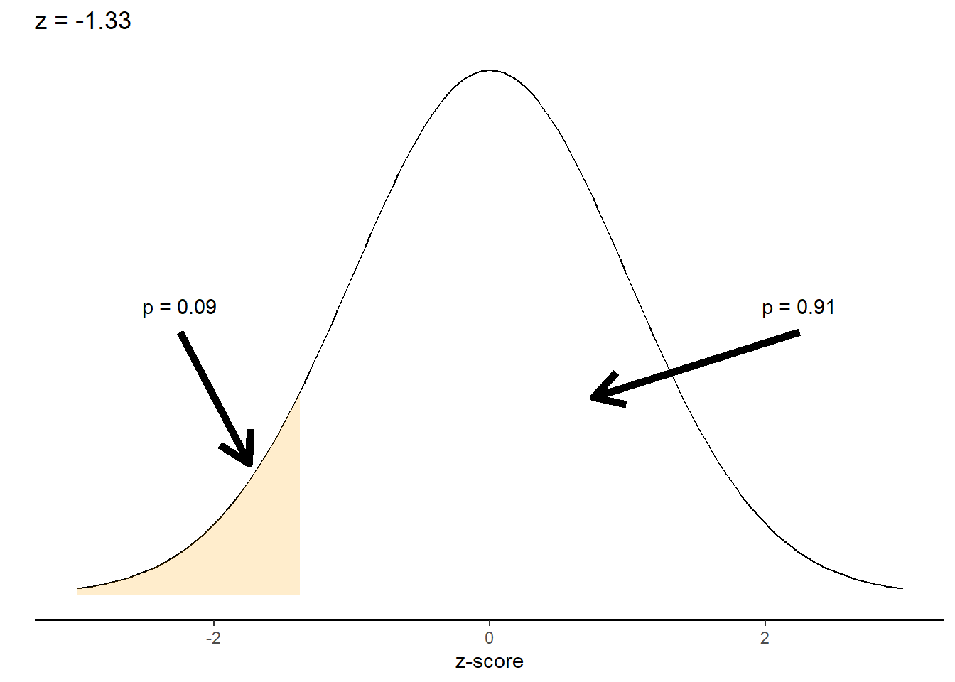
In Chapter 2, we were introduced to the normal distribution, one of the most widely used continuous distributions in statistics. We looked at an example of an N(42, 3) distribution, or a normally distributed population with a mean of 42 and a standard deviation of 3. We used the z-score calculation to determine that a value of interest, 38, was 1.33 standard deviations less than the mean. Similar to the dbinom() function, we can use the dnorm() function to find the density of the normal distribution given its mean and standard deviation:
dnorm(x = 38, mean = 42, sd = 3) ## [1] 0.05467002The pnorm() function finds the cumulative values for a normal distribution depending on the specified parameters.
pnorm(q = 38, mean = 42, sd = 3) ## [1] 0.09121122In other words, for an N(42, 3) distribution we can expect approximately 9% of observations to fall below 38. In contrast, its complement (or 91% of all observations) would be expected to be found greater than 38. This becomes more apparent after we plot it on the normal distribution:
To find the quantile function or a random number for the normal distribution, the qnorm() and rnorm() functions can be used. The same d, p, q, and r prefixes can be used for many other kinds of discrete and continuous distributions in R. For example, the dexp(), pexp(), qexp(), and rexp() functions can be used to determine the density, distribution, quantile, and random number for the exponential distribution.
In addition to the normal distribution, the cumulative distribution function will be valuable for calculating probabilities other continuous distributions as well. These include the Chi-square, uniform, exponential, and Weibull distributions.
3.5.1 Exercises
3.13 Historical data for the amount of lead in drinking water suggests its mean value is \(\mu = 6.3\) parts per billion (ppb) with a standard deviation of \(0.8\) parts per billion.
- An environmental specialist collects data on from 15 drinking water samples and calculates a mean lead content of 8.0 ppb. Is the mean of the specialist’s data unusually large?
- Use the
rnorm()function to create a series of 100 random numbers sampled from the drinking water data. - Make a histogram of the series of 100 random numbers using
ggplot()and describe the pattern you see.
3.14 Data from the Minnesota Department of Natural Resources in 2017 suggest the average mid-winter pack size of gray wolves (Canis lupus) has a mean of \(\mu = 4.8\) wolves with a standard deviation of \(\sigma = 1.5\) wolves. Use this information to answer the following questions.
- Assuming the pack sizes of wolves follows a normal distribution, calculate the probability of observing a pack size of two wolves. Would seeing this be a rare event?
- Calculate the probability of observing a wolf pack size between four and seven wolves.
3.6 Summary
Probabilities are so widespread that they come up in nearly every topic related to statistics. The five rules of probability can be used in future statistical calculations. While we focused extensively on the binomial and normal distribution in this chapter, there any many other kinds of discrete and continuous distributions that we can apply probabilities to. In the topic of hypothesis testing we will discuss p-values, or probability values, measures that assess the probability of obtaining a result under specific conditions. Having a solid grasp of probability is required as we continue applying these concepts of statistical inference.
3.7 References
Feller, W. 1968. An introduction to probability theory and its applications (Vol. 1). New York: Wiley. 509 p.
The old farmer’s almanac. 2020. How accurate is the Old Farmer’s Almanac weather forecast? Looking back on our winter 2019–2020 forecast, Available at: https://www.almanac.com/how-accurate-old-farmers-almanacs-weather-forecast
Stauffer, G.E., D.A. Miller, L.M. Williams, J. Brown. 2018. Ruffed grouse population declines after introduction of West Nile virus. Journal of Wildlife Management 82: 165–172.