Chapter 9 Multiple regression
9.1 Introduction
We have considered in detail the linear regression model in which a mean response is related to a single explanatory variable. Multiple linear regression will allow us to use two or more independent variables and employ least squares techniques to make appropriate inference. We’ve learned how to conduct hypothesis tests and calculate confidence intervals for coefficients such as \(\beta_1\) and \(\beta_2\) in a simple linear regression framework (i.e., the intercept and slope). This chapter will provide us the tools to understand the slopes associated with additional independent variables, e.g., \(\beta_2\), \(\beta_3\), and \(\beta_4\).
If you have more information that might help you to make a better prediction, why not use it? This is the value of multiple regression and why it is widely used in natural resources. There are several benefits of multiple linear regression, including:
- it allows us to use several variables to explain the variation in a single dependent variable,
- we can isolate the effect of a specific independent variable and see how it changes the predictions of a dependent variable, and
- we can control for other variables to see relationships between all variables.
Fortunately, the concepts of least squares apply as in simple linear regression. We can use many of the same functions in R for multiple linear regression that we’re familiar with.
9.2 Multiple linear regression
There are many problems in which knowledge of more than one explanatory variable is necessary to obtain a better understanding and more accurate prediction of a particular response. We will continue to use the concepts of least squares to minimize the residual sums of squares (SS(Res)) in multiple linear regression. The general model is written as
\[y = \beta_0 + \beta_1{x_1} + \beta_2{x_2} + ...+\beta_p{x_p} + \varepsilon\]
where \(\beta_0\) is the intercept, \(\beta_p\) are the “slopes” for each independent variable, and \(x_p\) are the pth independent variables. The least squares estimates for the coefficients \(\hat{\beta}_p\) involve more computations compared to simple linear regression. For \(p=2\) independent variables, we can calculate the coefficients \(\hat{\beta}_p\) if we know:
- the Pearson correlation coefficient r between all variables \(y, x_1, {\mbox{ and }}x_2\),
- the mean values of all variables \(\bar{y}, \bar{x}_1, {\mbox{ and }}\bar{x}_2\), and
- the sample standard deviations of all variables \(s_y, s_{x_1}, {\mbox{ and }} s_{x_2}\).
The formulas to calculate the least squares estimates of a multiple linear regression with \(p = 2\) dependent variables is
\[\hat{\beta}_0=\bar{y}-\hat{\beta}_1\bar{x}_1-\hat{\beta}_2\bar{x}_2\]
\[\hat{\beta}_1=\bigg(\frac{r_{y,x_1}-r_{y,x_2}r_{x_1,x_2}}{1-(r_{x_1,x_2})^2}\bigg)\bigg(\frac{s_y}{s_{x_1}}\bigg)\]
\[\hat{\beta}_2=\bigg(\frac{r_{y,x_2}-r_{y,x_1}r_{x_1,x_2}}{1-(r_{x_1,x_2})^2}\bigg)\bigg(\frac{s_y}{s_{x_2}}\bigg)\]
To understand the principles of multiple linear regression, consider data collected on peregrine falcons (Falco peregrinus). Data were simulated based on information presented in Kéry (2010) and include the following variables:
wingspan: the wingspan length measured in cm,weight: weight, measured in g,tail: tail length, measured in cm, andsex: sex of the falcon (female or male).
These attributes were measured on 20 falcons, presented in the falcon data set from the stats4nr package:
## # A tibble: 6 x 4
##   wingspan weight  tail sex
##      <dbl>  <dbl> <dbl> <chr>
## 1       96    950  15.5 F
## 2       97   1100  16.5 F
## 3      109   1295  17.6 F
## 4      110   1350  18.2 F
## 5       97   1150  16.6 F
## 6      102   1380  17.5 F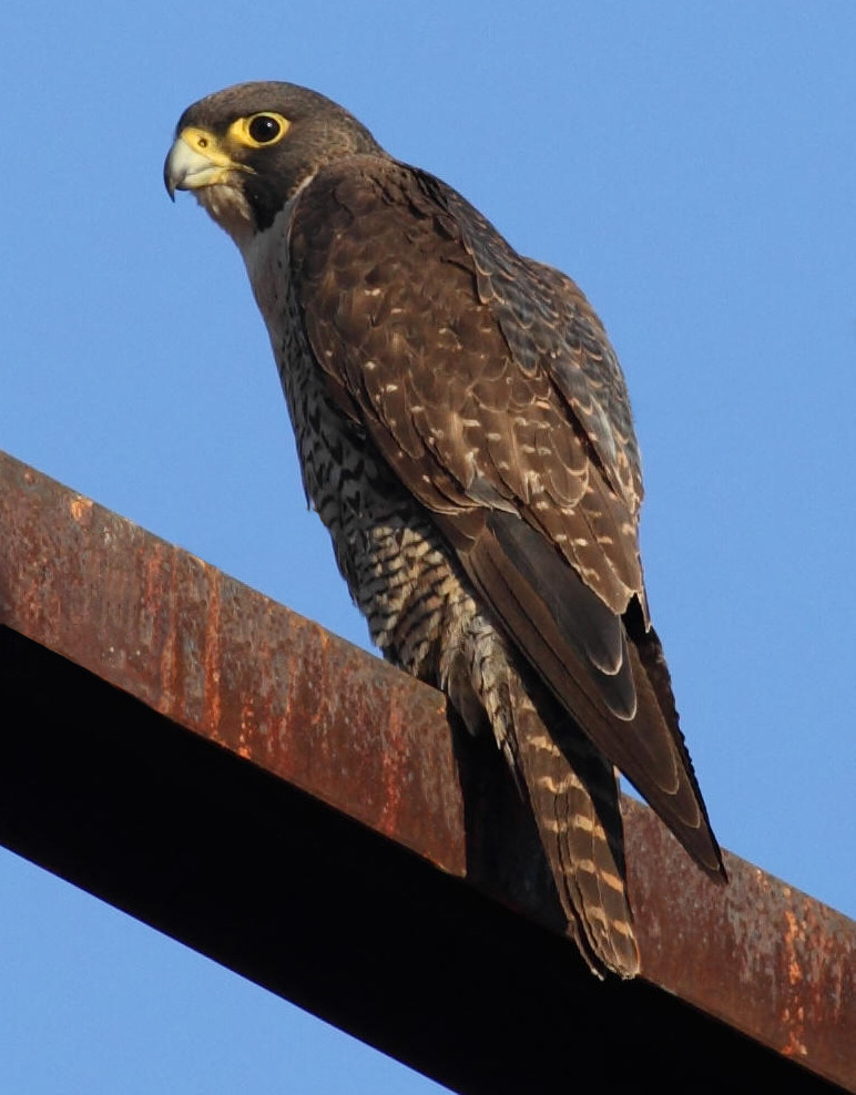
FIGURE 9.1: Peregrine falcon. Image: Christopher Watson.
Falcons are a sexually dimorphic species, indicating that females are larger than males. The following plot shows the distribution of falcon weights by sex using geom_density():
ggplot(falcon, aes(x = weight, col = sex)) +
        geom_density() +
        labs(x = "Falcon weight (g)")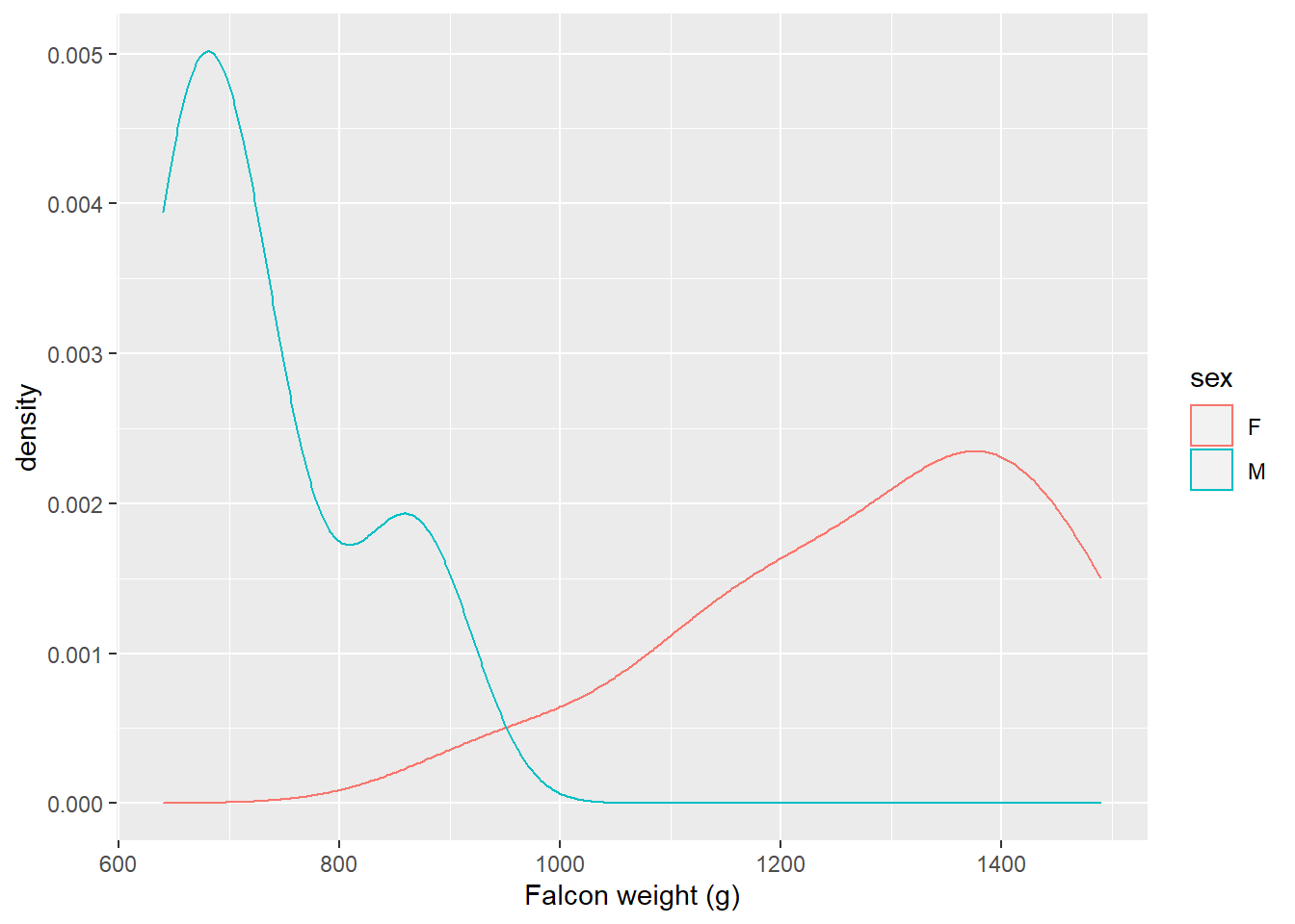
With multiple linear regression you likely have lots of variables, and it’s a good practice to start with visualizing them. The GGally package in R allows you to produce a matrix of scatter plots, distributions, and correlations among multiple variables. This is very useful in multiple regression when we might be interested in looking at a large number of variables and their relationships. The ggpairs() function provides this, and we can see the differences between male (M) and female (F) falcons:
install.packages("GGally")
library(GGally)ggpairs(falcon, aes(col = sex))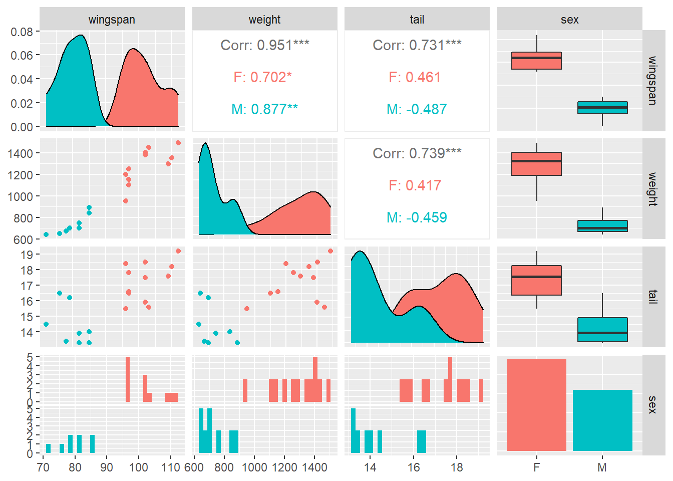
We are interested in predicting the wingspan length of these falcons. In addition to looking at the ggpairs() output, we find the correlation between wingspan and weight to be 0.95:
cor(falcon$wingspan, falcon$weight)## [1] 0.9512555So, there is a strong positive correlation between falcon wingspan length and weight. However there is still some variability that is not accounted for when investigating these two variables (Fig. 9.2).
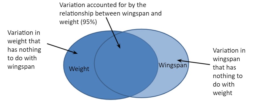
FIGURE 9.2: Two-way interactions between falcon weight and wingspan.
Consider another independent variable that might be useful: the length of the falcon’s tail. In addition to determining the correlation between wingspan and tail length (0.73), we also know the correlation between the two independent variables tail length and weight (0.74), and the correlation between wingspan and the “interaction” between tail length and weight (0.94):
cor(falcon$wingspan, falcon$tail)## [1] 0.7313432cor(falcon$weight, falcon$tail)## [1] 0.7385734cor(falcon$wingspan, falcon$tail*falcon$weight)## [1] 0.9406831These three-way interactions are summarized in Fig. 9.3, and you can see that adding additional independent variable captures more of the variability associated with the response variable.
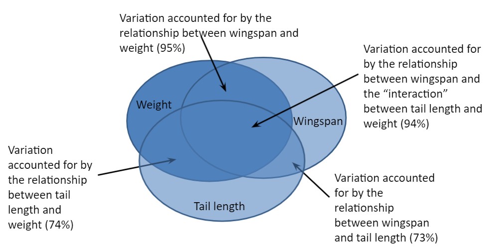
FIGURE 9.3: Three-way interactions between falcon weight, wingspan, and tail length.
As in simple linear regression, the method of least-squares for multiple linear regression chooses \(\hat\beta_0, \hat\beta_1, ... \hat\beta_p\) to minimize the sum of the squared deviations \((y_i-\hat{y}_i)^2\). The regression coefficients reflect the unique association of each independent variable with the response variable \(y\) and are analogous to the slopes in simple linear regression.
9.2.1 Implementation in R
In R, multiple linear regression can be specified by adding a + between all independent variables. We can perform a multiple linear regression using both weight and tail length to predict the wingspan of falcons:
falcon.lm <- lm(wingspan ~ weight + tail, data = falcon)
summary(falcon.lm)
##
## Call:
## lm(formula = wingspan ~ weight + tail, data = falcon)
##
## Residuals:
## Min 1Q Median 3Q Max
## -5.3103 -3.0005 -0.4342 2.3996 7.2011
##
## Coefficients:
## Estimate Std. Error t value Pr(>|t|)
## (Intercept) 48.514650 8.642648 5.613 3.10e-05 ***
## weight 0.035743 0.004342 8.232 2.47e-07 ***
## tail 0.408272 0.708697 0.576 0.572
## ---
## Signif. codes: 0 '***' 0.001 '**' 0.01 '*' 0.05 '.' 0.1 ' ' 1
##
## Residual standard error: 3.945 on 17 degrees of freedom
## Multiple R-squared: 0.9067, Adjusted R-squared: 0.8957
## F-statistic: 82.61 on 2 and 17 DF, p-value: 1.753e-09We can see that regression coefficients indicate falcon wingspans are longer on heavier birds with longer tail lengths. Note the p-value of 0.572 indicates tail length as a non-significant variable in the model, a finding we’ll revisit shortly.
Two other functions from the broom package allow you to extract important values from regression output. The tidy() function extracts the key values associated with the regression coefficients and places them in an R data frame stored as a tibble:
library(broom)
tidy(falcon.lm)
## # A tibble: 3 x 5
## term estimate std.error statistic p.value
## <chr> <dbl> <dbl> <dbl> <dbl>
## 1 (Intercept) 48.5 8.64 5.61 0.0000310
## 2 weight 0.0357 0.00434 8.23 0.000000247
## 3 tail 0.408 0.709 0.576 0.572The glance() function provides an R data frame containing the summary statistics of the model, such as \(R^2\) and \(R_{adj}^2\)
glance(falcon.lm)## # A tibble: 1 x 12
## r.squared adj.r.squared sigma statistic p.value df
## <dbl> <dbl> <dbl> <dbl> <dbl> <dbl>
## 1 0.907 0.896 3.94 82.6 1.75e-9 2
## # ... with 6 more variables: logLik <dbl>, AIC <dbl>,
## # BIC <dbl>, deviance <dbl>, df.residual <int>,
## # nobs <int>Similar to what we did in simple linear regression, the augment() function can be applied to the multiple regression object to view the residuals:
falcon.resid <- augment(falcon.lm)
head(falcon.resid)
## # A tibble: 6 x 9
## wingspan weight tail .fitted .resid .hat .sigma .cooksd
## <dbl> <dbl> <dbl> <dbl> <dbl> <dbl> <dbl> <dbl>
## 1 96 950 15.5 88.8 7.20 0.0574 3.62 0.0718
## 2 97 1100 16.5 94.6 2.43 0.0522 4.02 0.00736
## 3 109 1295 17.6 102. 7.01 0.0856 3.63 0.108
## 4 110 1350 18.2 104. 5.80 0.115 3.76 0.106
## 5 97 1150 16.6 96.4 0.603 0.0544 4.06 0.000474
## 6 102 1380 17.5 105. -2.99 0.105 3.99 0.0251
## # ... with 1 more variable: .std.resid <dbl>We can run the diagPlot() function presented in Chapter 8 to visualize the model’s diagnostic plots:
library(patchwork)

p.diag <- diagPlot(falcon.resid)

(p.diag$p.resid | p.diag$p.stdresid) /
(p.diag$p.srstdresid | p.diag$p.cooks)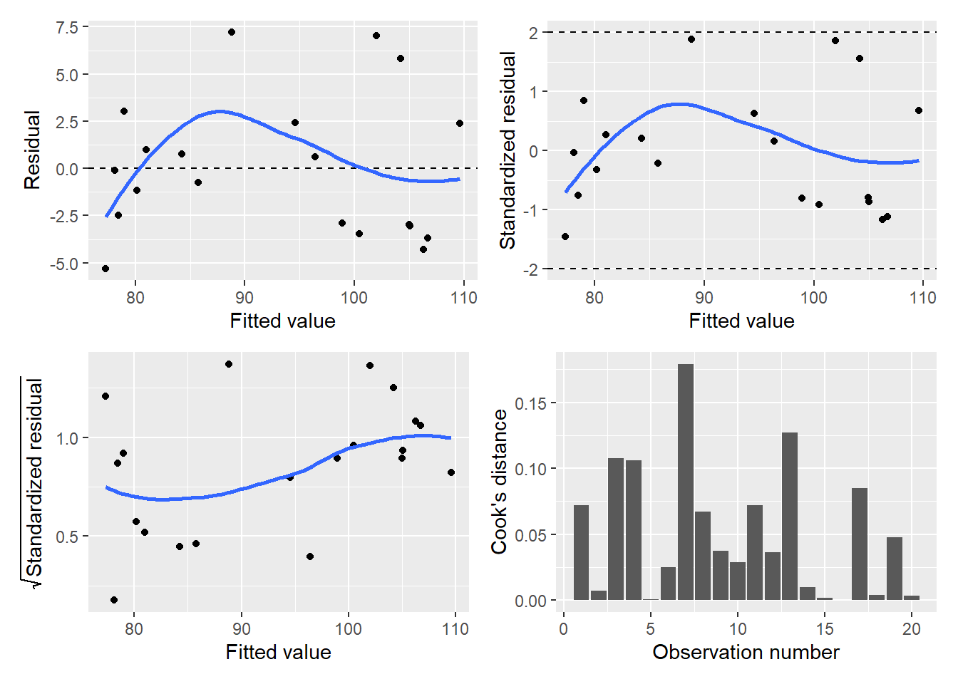
The residual and other diagnostic plots look satisfactory for this multiple linear regression. There is a slight trend in larger values for residuals as fitted values increase which may provide some justification for transforming the data. For the purpose of illustration, we’ll continue to investigate the output from the falcon.lm regression.
9.2.2 Inference in multiple regression
Recall we can calculate confidence intervals to inform us about the population means of the regression coefficients. To understand the confidence intervals of \(\beta_0, \beta_1, ... \beta_p\), we rely again on the t distribution, with \(n – p – 1\) degrees of freedom. The confint() function also provides the confidence intervals for multiple linear regression objects:
confint(falcon.lm)## 2.5 % 97.5 %
## (Intercept) 30.280257 66.7490436
## weight 0.026582 0.0449045
## tail -1.086948 1.9034918We can use the ANOVA table to partition the variance of a multiple linear regression model. The greatest difference compared to simple linear regression is the degrees of freedom for the regression and residual components, which depends on p, the number of predictors used in the regression.
| Source | Degrees of freedom | Sums of squares | Mean square | F |
|---|---|---|---|---|
| Regression | p | SS(Reg) | MS(Reg) = SS(Reg)/p | MS(Reg) / MS(Res) |
| Residual | n-p-1 | SS(Res) | MS(Res) = SS(Res)/n-p-1 |
|
| Total | n-1 | TSS |
|
|
The anova() function in R produces the ANOVA table. Consider the falcon wingspan regression:
anova(falcon.lm)## Analysis of Variance Table
##
## Response: wingspan
## Df Sum Sq Mean Sq F value Pr(>F)
## weight 1 2566.08 2566.08 164.8921 3.546e-10 ***
## tail 1 5.16 5.16 0.3319 0.5721
## Residuals 17 264.56 15.56
## ---
## Signif. codes: 0 '***' 0.001 '**' 0.01 '*' 0.05 '.' 0.1 ' ' 1Note that the function provides two rows for weight and tail that can be added together to calculate the \(SS(Reg)\) and \(MS(Reg)\) values.
In multiple regression, the F-statistic follows an \(F(p, n − p − 1)\) distribution and tests the null hypothesis
\[H_0: \beta_1 = \beta_2 = ... =\beta_p\] versus the alternative hypothesis
\[{\mbox{At least one }} \beta_p \ne 0\]
A rejection of the null hypothesis and a significant p-value in multiple linear regression should be interpreted carefully. This does not mean that all p explanatory variables have a significant influence on your response variable, only that at least one variable does. The falcon output is a good example of this: the overall F-statistic is 82.61 indicating a rejection of the null hypothesis for the multiple linear regression. However, we see that weight is the only significant variable in the model at the \(\alpha=0.05\) level and tail is not.
When developing regression models, you should subscribe to the Albert Einstein quote: “Everything should be made as simple as possible, but no simpler.” Statisticians and data analysts term these parsimonious models, or models that achieve maximum prediction capability with the minimum number of independent variables needed. The next section discusses how to perform linear regression when you have a large number of independent variables available.
9.2.3 Exercises
9.1 The fish data set contains measurements on fish caught in Lake Laengelmavesi, Finland (Puranen 1917). The data include measurements from seven species where the weight, length, height, and width of fish were measured. The variables are defined as:
Species: (Fish species name)Weight: (Weight of the fish [grams])Length1: (Length from the nose to the beginning of the tail [cm])Length2: (Length from the nose to the notch of the tail [cm])Length3: (Length from the nose to the end of the tail [cm])Height: (Maximal height as % of Length3)Width: (Maximal width as % of Length3)
Read in the data set from the stats4nr package and explore the data using the
ggpairs()function from the GGally package. Add a different color to your plot for each of the seven species. What do you notice about the relationships between the three length variables? Which fish species has the largest median value for width?Create a new data set called perch that contains only observations of perch species using the
filter()function. Then, uselm()to create a simple linear regression with this data set to predictWeightusingLength3as an independent variable (the length from the nose to the end of the tail). Usesummary()on the model to investigate its performance. How much would a perch with aLength3of 30 cm weigh?Apply the
diagPlot()function to the simple linear regression model. What is the general trend in the residual plot? Which assumption of regression is violated here and what indicates this violation?To remedy the regression, create a new variable in the perch data set called
Length3sqthat squares the value ofLength3. In addition, create a new variable by log-transforming the response variableWeight. Then, perform a multiple linear regression using bothLength3andLength3sqto predict the log-transformed weight. Then, provide the output for the residual plot for this model. What has changed about the characteristics of the residual plot? What can you conclude about the assumptions of this regression?Use the
glance()function from the broom package to compare the adjusted R-squared values between the simple and multiple linear regression models.
9.2 This question performs a multiple linear regression using the falcon data set.
“Dummy” variables, or indicator variables, are dichotomous indicators of a variable used in a regression. Create a new dummy variable in the falcon data set that creates a numeric 1,0 variable that represents whether a falcon is male or female. Then, perform a multiple linear regression predicting
wingspanusingweightand the dummy variable for sex of the falcon. Do you reject or fail to reject the null hypothesis that all slopes \(\beta_p\) are equal to zero at the \(\alpha = 0.05\) level?Use the
tidy()function on the multiple linear regression to extract the regression coefficients.Provide 85% confidence intervals for the regression coefficients in this model.
9.3 All subsets regression
In many natural resources data sets, dozens of independent variables might be available that are related to your response variable of interest. We might be interested in predicting our response variables by testing the performance of linear regressions using all of these variables. However, there may be a lot of different combinations of all possible regressions to do, so many that we don’t want to fit an lm() model for each of them. That would take too much time!
The leaps package in R searches for the best subsets of all variables that might be used in a multiple linear regression:
install.packages("leaps")
library(leaps)
We can use the regsubsets() function from the package to run all subsets regression predicting a response variable of interest. For example, consider the falcon data set. We create the falcon.leaps object using the function, which appears similar to the lm() function:
falcon.leaps <- regsubsets(wingspan ~ weight + tail + factor(sex),
                           data = falcon)
We can plot the \(R_{adj}^2\) values for all subsets using the plot() function:
plot(falcon.leaps, scale="adjr2")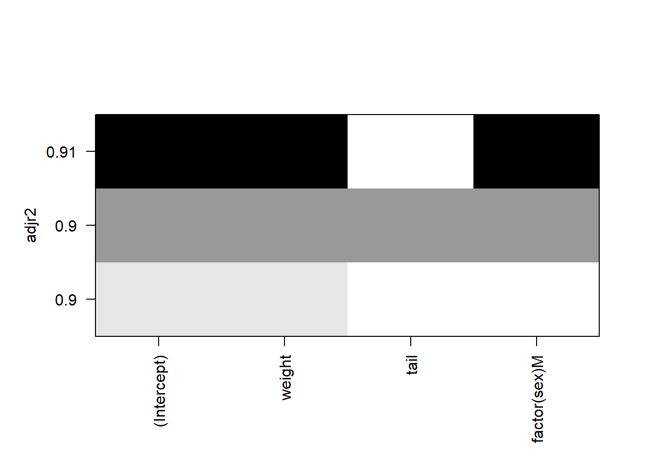
FIGURE 9.4: Plot showing adjusted R-squared values from the leaps package.
In the plot, each row represents a model. The models are ranked from the highest \(R_{adj}^2\) on the top to the lowest on the bottom. In this falcon example, the regression subset indicates that a model with an intercept, weight, and sex of the falcon performs best (e.g., it provides the highest \(R_{adj}^2\) ). The shading color is related to the significance level of the variables, with darker colors indicating lower p-values.
9.3.1 Stepwise regression
Stepwise regression techniques involve using an automated process to select which variables to include in a model. Two stepwise techniques involve forward (beginning with a null model and adding variables) and backward regression (beginning with all variables in a model and subsequently removing them). The general approach in a stepwise regression is to set a significance level \(\alpha\) for deciding when to enter a predictor into the model. We also set a significance level for deciding when to remove a predictor from the model. The values chosen for \(\alpha\) are typically 0.15 or less.
To select a subset of predictors from a larger set, we’ll use the step() function in R to help with this. First, we’ll fit a null model for the falcon data set using no predictors for wingspan:
null <- lm(wingspan ~ 1, data = falcon)Then, we’ll fit a full model, using all possible predictors of wingspan:
full <- lm(wingspan ~ weight + tail + factor(sex), data = falcon)The step() function can be used to implement forward regression using direction = "forward". In this approach, we begin with no variables in the model and proceed forward, adding one variable at a time. The R output displays the forward regression process:
step(null, scope = list(lower = null, upper = full),
     direction = "forward")
## Start: AIC=101.09
## wingspan ~ 1
##
## Df Sum of Sq RSS AIC
## + weight 1 2566.1 269.72 56.033
## + factor(sex) 1 2332.0 503.79 68.529
## + tail 1 1516.8 1319.04 87.778
## <none> 2835.80 101.087
##
## Step: AIC=56.03
## wingspan ~ weight
##
## Df Sum of Sq RSS AIC
## + factor(sex) 1 36.974 232.75 55.084
## <none> 269.72 56.033
## + tail 1 5.165 264.56 57.646
##
## Step: AIC=55.08
## wingspan ~ weight + factor(sex)
##
## Df Sum of Sq RSS AIC
## <none> 232.75 55.084
## + tail 1 0.036654 232.71 57.081##
## Call:
## lm(formula = wingspan ~ weight + factor(sex), data = falcon)
##
## Coefficients:
## (Intercept) weight factor(sex)M
## 65.6764 0.0282 -6.4069At each step, output shows the Akaike’s information criterion (AIC), a measure of prediction error that measures the quality of a model. Models with lower AIC values are ideal, and a model will be preferred over another if the difference in AIC is less than two units. Also shown are the sums of squares and residual sums of squares as each variable is added to the model. The coefficients listed at the end of the output indicate that in addition to the intercept, weight and sex are the variables chosen in the forward regression.
The step() function can also be used to implement backward regression (direction = "backward"). In this approach, we start with all potential variables in the model and proceed backward, removing one variable at a time:
step(full, direction = "backward")## Start: AIC=57.08
## wingspan ~ weight + tail + factor(sex)
##
## Df Sum of Sq RSS AIC
## - tail 1 0.037 232.75 55.084
## <none> 232.71 57.081
## - factor(sex) 1 31.846 264.56 57.646
## - weight 1 261.916 494.63 70.161
##
## Step: AIC=55.08
## wingspan ~ weight + factor(sex)
##
## Df Sum of Sq RSS AIC
## <none> 232.75 55.084
## - factor(sex) 1 36.974 269.72 56.033
## - weight 1 271.044 503.79 68.529##
## Call:
## lm(formula = wingspan ~ weight + factor(sex), data = falcon)
##
## Coefficients:
## (Intercept) weight factor(sex)M
## 65.6764 0.0282 -6.4069Note that the backward regression approach identifies the same variables as the forward regression.
DATA ANALYSIS TIP: Generally, if you have a very large set of predictors (say, greater than five) and are looking to identify a few key variables in your model, forward regression is best. If you have a modest number of predictors (less than five) and want to eliminate a few, use backward regression.
9.3.2 Evaluating multiple linear regression models
Multiple linear regression models can become unwieldy as you add numerous independent variables to your model. For example, you may be using too many variables in your model such that they are correlated with one another. This is termed multicollinearity, i.e., when one variable is held constant, another is in effect also held constant. Multicollinearity is a topic that needs to be addressed in analyses of multiple linear regression.
The consequences of not addressing multicollinearity can be serious. These include (1) a final model with regression coefficients that have large uncertainty and (2) an inaccurate representation of the sums of squares for regression and residual components. The primary solutions for avoiding multicollinearity include (1) removing some of the independent variables and (2) fitting separate models with each independent variable.
The variance inflation factor (VIF) is a useful metric that evaluates the degree of multicollinearity in a regression model. The greater the VIF, the greater the collinearity between variables. A VIF for a single independent variable is obtained using the \(R^2\) of the regression of that variable compared to all other independent variables. Generally, VIF values greater than 10 indicate a need to reevaluate which independent variables are used in the regression.
The car package was developed to accompany a textbook on regression and contains useful functions for regression (Fox and Weisberg 2009). We will install the package and load it with library() so that we can look at some of the functions that are contained within it.
install.packages("car")

library(car)
We can determine VIF using the vif() function available in the car package for the full model with three variables predicting falcon wingspan:
vif(full)## weight tail factor(sex)
## 5.492267 2.495839 6.045090The VIF values are all less 10, indicating no serious multicollinearity present. You can see the values for VIF decrease when you evaluate the reduced model using only weight and sex:
reduced <- lm(wingspan ~ weight + factor(sex), data = falcon)

vif(reduced)
## weight factor(sex)
## 5.328972 5.3289729.3.3 Exercises
9.3 Recall the elm data set on cedar elm trees located in Austin, Texas to answer the following questions.
Read in the data set and explore the data using the
ggpairs()function. What do you notice about the distribution ofDIAandHT? What is the correlation coefficient betweenHTandCROWN_DIAM_WIDE?Create a new dummy variable in the elm data set that creates a {1,0} variable that represents how much light a tree receives. If it is an open-grown or dominant tree (i.e., a
CROWN_CLASS_CDof 1 or 2), the tree will have a 1 for the dummy variable. These trees are receiving a lot of light. If it is a co-dominant, intermediate, or overtopped tree (i.e., aCROWN_CLASS_CD of 3, 4, or 5), the tree will have a 0 for the dummy variable. These trees have some or no light available to them. How many trees are in each category?We might be interested in predicting elm tree heights (
HT) using all of these variables. Use theregsubsets()function to run all subsets regression predictingHTusing the independent variablesDIA,CROWN_HEIGHT,CROWN_DIAM_WIDE,UNCOMP_CROWN_RATIO, and the dummy variable you made for CROWN_CLASS_CD (a factor variable). Visualize the results by plotting the \(R_{adj}^2\) for all models using theplot()function. What is the \(R_{adj}^2\) for this model? Which variables are chosen in the best performing model?Fit both forward and backward regressions considering all variables to predict
HT. Which variables are selected by the forward and backward regression techniques? Are these the same sets of variables? Explain why they may or may not be the same.Calculate the variance inflation factor for the variables identified in the backward selection process. Are you concerned that multicollinearity is present in the model?
9.4 Let’s revisit the perch data set. Fit a regression model that predicts the weight of perch using the independent variables Length1, Length2, and Length3 and calculate the variance inflation factor. Are you concerned with multicollinearity and/or variance inflation in this model?
9.4 Summary
Multiple regression techniques allow us to consider more than one independent variable to make a prediction on our response variable of interest. Similar to simple linear regression, the lm() function can be used to fit multiple regression models. Stepwise regression techniques allow us to identify which variables are best to include in our regression models through an automated process, without the need to fit subsets of models using different combinations of independent variables. This allows us to “prune” our variables to result in only the most important ones, however, some cautions need to be recognized when fitting multiple linear models.
Multicollinearity is a widespread concern in many biological and natural resources data sets. Any analysis using multiple predictor variables in a modeling framework should evaluate multicollinearity. For making comparisons between multiple linear regression models, evaluation statistics such as \(R_{adj}^2\) and AIC are useful metrics.
9.5 References
Fox, J., S. Weisberg. 2019. An R companion to applied regression, 3rd ed. Sage. 608 p.
Kéry, M. 2010. Introduction to WinBUGS for ecologists. Academic Press. 302 p.
Puranen, J. 1917. Fish catch data set. Journal of Statistics Education, Data Archive: Available at: http://jse.amstat.org/datasets/fishcatch.txt