Chapter 12 Logistic regression
12.1 Introduction
One of the primary assumptions of the regression techniques we have learned up to this point is that the response variables are independent normal random variables, i.e., the normality assumption. Similarly, linear models using ordinary least squares regression are not appropriate when the response \(y_i\) is stored as a binary or count variable or when the variance of \(y_i\) depends on the mean. For example, the relationship between the size of an organism and its age is curved, i.e., growth tends to rise in juvenile stages, flatten out, and possibly decline after that.
This chapter will discuss how generalized linear models can be used to perform logistic regression (when the response variable is a binary variable), multinomial logistic regression (when there are three or more categorical variables for the response variable), and ordinal regression (when there are three or more categorical variables for the response variable and they are ordered or ranked in a meaningful way).
12.2 An overview of generalized linear models
Generalized linear models (GLMs) extend the linear modeling framework to response variables that are not normally distributed. The GLM framework generalizes linear regression by allowing the linear model to be related to the response variable by using a link function. The link function describes the relationship between the linear predictor and its mean value, while a variance function describes the relationship between the variance and mean. A GLM model can be broadly written as
\[\eta_i=\beta_0+\beta_1x_{i1}+\beta_2x_{i2}+...+\beta_kx_{ik}\]
where \(\eta_i\) represents the linear predictor, \(\beta_i\) represent parameters, and \(x_i\) represent independent variables.
The appropriate link function to specify relies on how best to describe the error distribution in the model. Three common link functions used with natural resources data include the Gaussian, binomial, and Poisson types. The Gaussian link function is most similar to linear regression techniques where data are distributed normally with a range of negative and positive values. The binomial link function is used when the response variable is categorical, e.g., a binary or multinomial variable. A binomial count could also consist of the number of “yes” occurrences out of N “yes/no” occurrences. A Poisson link function is used with count data where the response variable is stored as an integer, e.g., 0, 1, 2, 3, etc.
In R, the glm() function fits GLMs. The function is similar to lm(), which is used in regression and analysis of variance. The main difference is that we need to include an additional argument that describes the error distribution and link function to be used in the model. In the family = statement within glm(), the link functions for the Gaussian, binomial, and Poisson types can be specified as link = identity, link = logit, and link = log, respectively.
| Family | Link function | Data | Example |
|---|---|---|---|
| Gaussian | Identity | Normally distributed data | Height of a plant |
| Binomial | Logit | A binary or multinomial variable | Whether a plant is alive or dead |
| Poisson | Log | Count data (e.g., 0, 1, 2, 3) | Number of plants in a square meter plot |
12.2.1 Logistic regression
Logistic regression is one of the most common types of GLMs. Logistic regression analyzes a data set in which there are one or more independent variables that determine an outcome. This differs greatly from linear regression because in logistic regression, the dependent variable is categorical. Hence, logistic regression models a binomial count, e.g., the number of “yes” or “no” occurrences.
Concepts presented in Chapters 5 and 6 deal with hypothesis tests of count and proportional data, however, logistic regression will allow you to model the probability of a binomial count occurring with a suite of predictors. In natural resources, logistic regression is often used to quantify the presence/absence of some phenomenon or the living status of an organism (e.g., alive or dead).
We learned that the logit link function can be used to model a binary variable. A logistic regression model is written as:
\[\mbox{logit}(p)=\beta_0+\beta_1x_{1}+\beta_2x_{2}+...+\beta_kx_{k}\]
The logit function relies on knowing the probability of success \(p\) and dividing it by its complement \(1-p\), or the probability of failure. The odds ratio is often presented as a log odds after taking its logarithm. In doing this, log odds have values centered around zero:
\[\mbox{logit}(p)=\mbox{log}{\frac{p}{1-p}}\]
For example, consider that 65% of trees in a forest were defoliated by an insect. The odds ratio would be \(0.65/0.35 = 1.85\) and a log odds ratio of \(\mbox{log}(0.65/0.35) = 0.62\). Values with negative log odds are associated with probabilities of success less than 0.50 and values with positive log odds are associated with probabilities of success greater than 0.50.
| Probability | Odds | Log odds |
|---|---|---|
| 0.05 | 0.05 | -3.00 |
| 0.25 | 0.33 | -1.11 |
| 0.50 | 1.00 | 0.00 |
| 0.75 | 3.00 | 1.10 |
| 0.95 | 19.00 | 2.94 |
Logistic regression is fit with maximum likelihood techniques using one or more independent variables. Similar to how we can evaluate multiple regression models, the Akaike’s information criterion (AIC) can be used to evaluate the quality of logistic regression models. The AIC is calculated as:
\[\mbox{AIC} = 2k - 2ln(\hat{L})\]
where \(L\) represents the maximum value for the likelihood of the model and \(k\) represents the number of parameters in the model. The AIC value can be compared across different models fit to the same dependent variable. A lower AIC for a model indicates a higher-quality model if a difference of two or more units is observed.
12.2.1.1 Case study: Predicting deer browse on tree seedlings
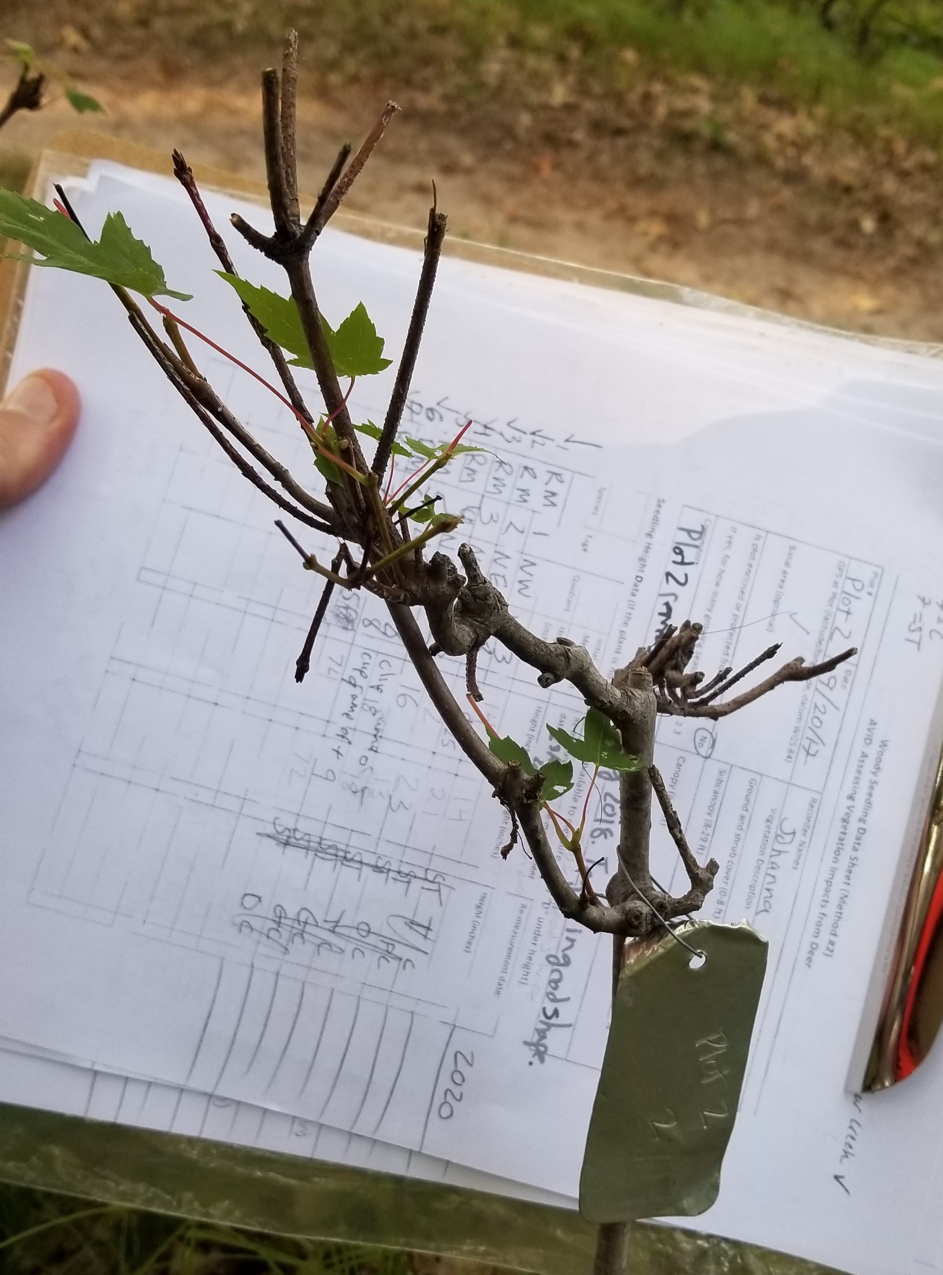
FIGURE 12.1: Tree seedling showing evidence of continual browse damage from white-tailed deer. Photo by the author.
To see how logistic regression is implemented in R, an experiment that planted oak (Quercus) trees in fenced and non-fenced areas was conducted at the Cloquet Forestry Center in Cloquet, MN. In this region, oak seedlings are palatable to white-tailed deer (Odocoileus virginianus) that use them as a food source. In addition to fencing, oaks were planted close together to minimize risk from deer browse. This experiment was based on the German “Truppflanzungs” idea of the 1970s (Saha et al. 2017). Oak seedlings were planted in tight clusters with 20 to 30 individuals per square meter. The goal of the experiment was to provide conditions so that at least one tree per cluster would survive and thrive in forests subject to severe herbivory pressure from white-tailed deer.
The data are found in the trupp data set in the stats4nr R package. There are nine variables and 762 observations in the data:
library(stats4nr)

trupp
## # A tibble: 762 x 9
## plot trmt tree year dia ht browse dead missing
## <chr> <chr> <dbl> <dbl> <dbl> <dbl> <dbl> <dbl> <dbl>
## 1 P1 FENCE 1 2007 0 0 0 1 0
## 2 P1 FENCE 2 2007 8.7 47 0 0 0
## 3 P1 FENCE 3 2007 6.7 65 0 0 0
## 4 P1 FENCE 4 2007 7.6 41 0 0 0
## 5 P1 FENCE 5 2007 6.2 26 0 0 0
## 6 P1 FENCE 6 2007 4.9 33 0 0 0
## 7 P1 FENCE 7 2007 9.2 46 0 0 0
## 8 P1 FENCE 8 2007 8.3 45 0 0 0
## 9 P1 FENCE 9 2007 6.3 46 0 0 0
## 10 P1 FENCE 10 2007 8.5 62 0 0 0
## # ... with 752 more rowsThe variables are:
plot: Plot identification numbertrmt: Fencing treatment (FENCE, NOFENCE, CTRL)tree: Tree identification numberyear: Year of measurement (2007, 2008, or 2013)dia: Seedling diameter (mm)ht: Seedling height (cm)browse: Indicator for whether or not seedling was browsed (1) or not (0)dead: Indicator for whether or not seedling was dead (1) or not (0)missing: Indicator for whether or not seedling was missing (1) or not (0)
Our interest is in predicting whether or not an oak seedling was browsed based on its diameter and whether it was located in the fenced treatment. Prior to performing the logistic regression, we will remove the control plots to directly compare the fenced and non-fenced treatments:
trupp <- trupp %>%
  filter(trmt != "CTRL")
The data result in 522 observations. To visualize the results, we can see that seedlings in fenced areas tend to be browsed less (browse = 0) and are larger in diameter than non-fenced seedlings:
p.browse <- ggplot(trupp, aes(dia, browse, col = trmt)) +
  geom_point() +
  labs(x= "Diameter (mm)", y = "P(browse)")
p.browse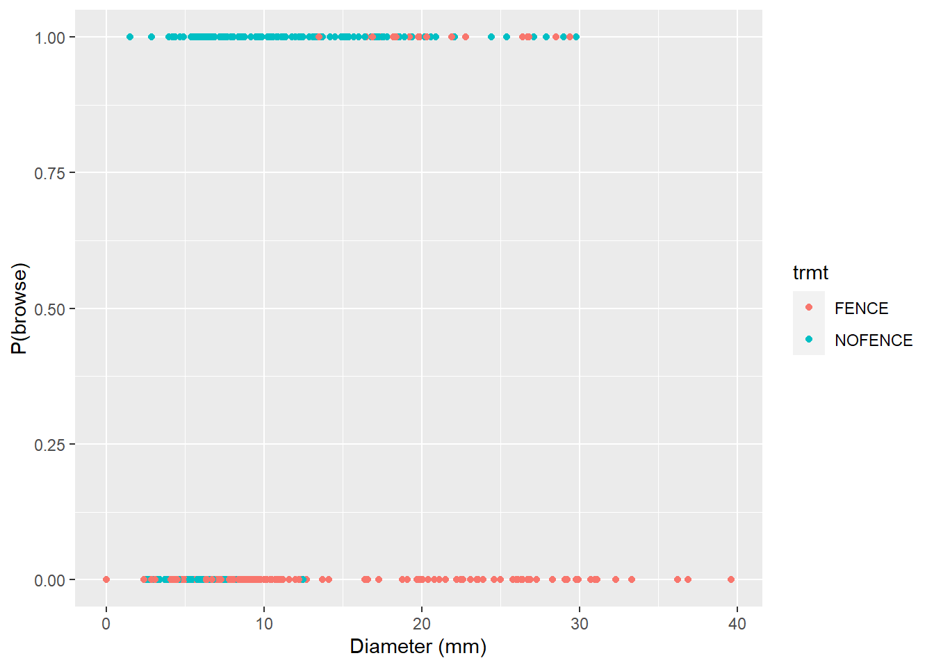
The glm() function in R is used to specify a logistic regression. We model the response variable browse using the predictor variables dia and trmt. We specify the logit link function within the family statement to indicate a binary response in our model:
browse.m1 <- glm(browse ~ dia + trmt,
                 family = binomial(link = 'logit'),
                 data = trupp)
summary(browse.m1)
##
## Call:
## glm(formula = browse ~ dia + trmt, family = binomial(link = "logit"),
## data = trupp)
##
## Deviance Residuals:
## Min 1Q Median 3Q Max
## -2.1313 -0.7953 -0.1212 0.5361 3.0946
##
## Coefficients:
## Estimate Std. Error z value Pr(>|z|)
## (Intercept) -6.37547 0.69352 -9.193 < 2e-16 ***
## dia 0.21560 0.02696 7.998 1.26e-15 ***
## trmtNOFENCE 4.77196 0.53263 8.959 < 2e-16 ***
## ---
## Signif. codes: 0 '***' 0.001 '**' 0.01 '*' 0.05 '.' 0.1 ' ' 1
##
## (Dispersion parameter for binomial family taken to be 1)
##
## Null deviance: 645.02 on 521 degrees of freedom
## Residual deviance: 389.98 on 519 degrees of freedom
## AIC: 395.98
##
## Number of Fisher Scoring iterations: 6The summary output provides the deviance residuals, coefficients, and AIC value for the logistic model. The residual deviance measure is analogous to the residual sums of squares metric used in linear regression. The predictor variables dia and trmt are statistically significant and their coefficients provide the change in the log odds of the browse. For interpretation, for every one-millimeter change in dia, the log odds of browse increases by 0.22. For seedlings in non-fenced areas, the log odds of browse increases by 4.77.
The log odds provided in R output for a logistic regression model is helpful but not easily interpreted. You can exponentiate the coefficients to determine the odds ratios directly:
exp(coef(browse.m1))## (Intercept) dia trmtNOFENCE
## 1.702813e-03 1.240605e+00 1.181504e+02So, for a one-unit increase in dia, the odds of an oak seedling being browsed increases by a factor of 1.24. For seedlings in non-fenced areas, the odds of them being browsed increases by a factor of 118. The conclusions of the experiment are that seedlings with a larger diameter that are found in non-fenced areas have a greater probability of being browsed.
12.2.1.2 Logistic regression from a 2x2 table
The trupp data set is formatted “long” such that each row contains a seedling observation. When dealing with binary outcomes in logistic regression, it is also common to record data in a 2x2 contingency table with the number of observations in each cell. This is especially useful when dealing with categorical predictor variables (e.g., trmt in the trupp data). However, applications with continuous predictor variables that vary for each observation (e.g., dia in the trupp data) require them to be organized in a long format for logistic regression.
For categorical variables, a logistic regression can be performed on data organized in a 2x2 contingency table. Data could be entered manually in this format (see Chapter 5 and the matrix() function) or an existing long data set can be modified into a 2x2 table using the with() and table() functions. For example, a new data set with trmt and browse as row and column name labels can be created from the trupp data set containing the number of observations in each category:
trupp.table <- with(trupp, table(trmt, browse))
trupp.table
## browse
## trmt 0 1
## FENCE 242 19
## NOFENCE 119 142To perform a logistic regression on this data set, adding the weights = Freq statement to the glm() function tells R to use the counts of observations in the model fitting:
browse.m2 <- glm(browse ~ trmt, weights = Freq,
                 family = binomial(link = 'logit'),
                 data = trupp.table)
summary(browse.m2)
##
## Call:
## glm(formula = browse ~ trmt, family = binomial(link = "logit"),
## data = trupp.table, weights = Freq)
##
## Deviance Residuals:
## 1 2 3 4
## -6.048 -13.672 9.978 13.148
##
## Coefficients:
## Estimate Std. Error z value Pr(>|z|)
## (Intercept) -2.5445 0.2383 -10.68 <2e-16 ***
## trmtNOFENCE 2.7212 0.2687 10.13 <2e-16 ***
## ---
## Signif. codes: 0 '***' 0.001 '**' 0.01 '*' 0.05 '.' 0.1 ' ' 1
##
## (Dispersion parameter for binomial family taken to be 1)
##
## Null deviance: 645.02 on 3 degrees of freedom
## Residual deviance: 495.94 on 2 degrees of freedom
## AIC: 499.94
##
## Number of Fisher Scoring iterations: 6An interested learner might try fitting the same logistic regression model using the trupp data set, which would yield identical results compared to the browse.m2 model. By adding more categorical variables as predictors and including their interactions, it is possible to extend the logistic regression model. Then, the quality of multiple logistic regression models could be compared using AIC.
12.2.1.3 Visualizing results and making predictions
We can modify the p.browse figure by adding the logistic curves for fenced and non-fenced areas. In ggplot() the stat_smooth() statement can include GLM model types if the binomial family is specified:
p.browse +
  stat_smooth(method = "glm", se = FALSE,
method.args = list(family = binomial)) 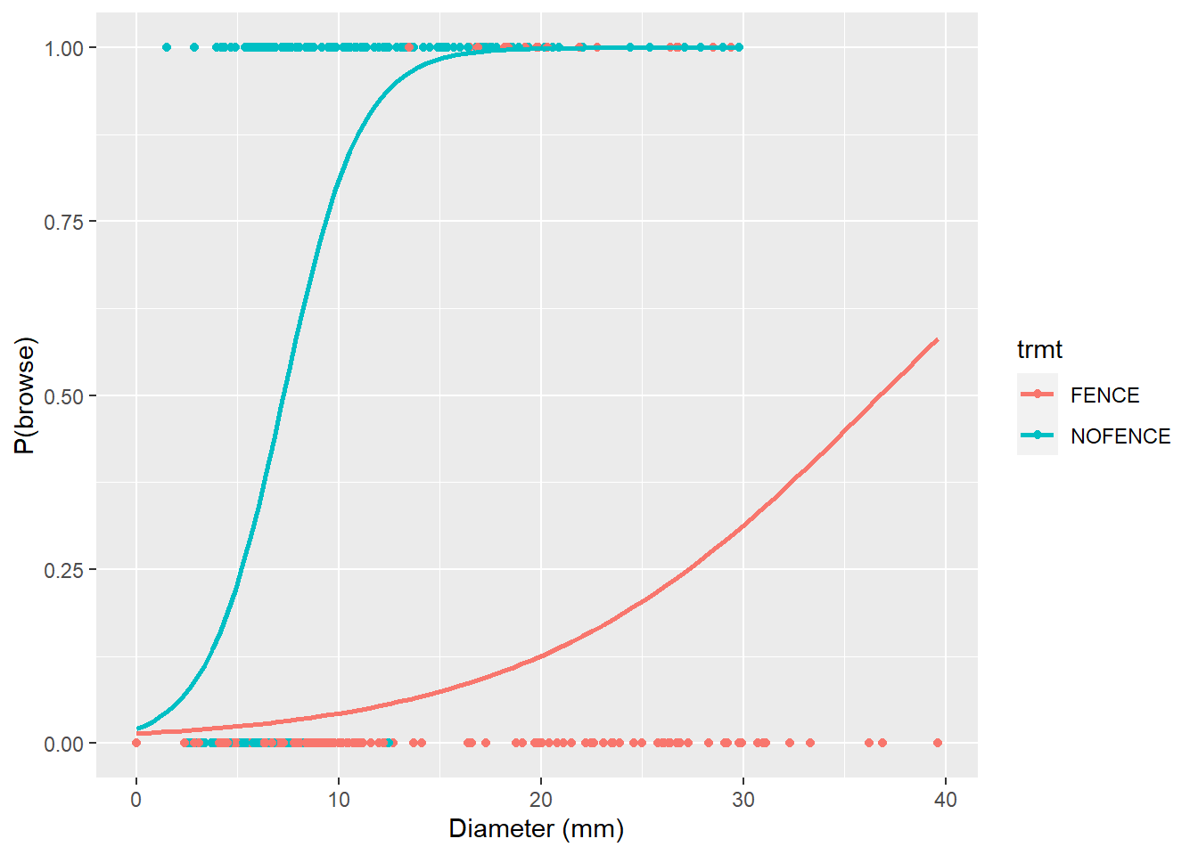
Here we can see the clear effects that fencing has in lowering the probability of deer browse on oak seedling. If we have new seedling observations and we seek to predict the probability of deer browse, the handy predict() function works well. For example, consider we have the following six seedlings and we want to estimate the probability of them being browsed:
new.seedling <- tibble(
  dia = c(10, 10, 20, 20, 30, 30),
  trmt = c("FENCE", "NOFENCE", "FENCE",
           "NOFENCE", "FENCE", "NOFENCE"))
We add a new variable termed P_browse which indicates the probability of a seedling being browsed. Specifying type = "response" provides the predicted probability:
new.seedling <- new.seedling %>%
  mutate(P_browse = predict(browse.m1,
                            newdata = new.seedling,
                            type = "response"))
new.seedling
## # A tibble: 6 x 3
## dia trmt P_browse
## <dbl> <chr> <dbl>
## 1 10 FENCE 0.0145
## 2 10 NOFENCE 0.635
## 3 20 FENCE 0.113
## 4 20 NOFENCE 0.938
## 5 30 FENCE 0.523
## 6 30 NOFENCE 0.99212.2.1.4 Assessing accuracy with the confusion matrix
Accuracy and error are two key metrics when using logistic regression to classify data. You can interpret the performance of the model much more deeply if you learn more about another valuable tool: the confusion matrix.
The confusion matrix includes rows and columns for all possible labels in a classification:
- True positives (TP): The model correctly predicts a positive value.
- True negatives (TN): The model correctly predicts a negative value.
- False positives (FP): The model incorrectly predicts a positive value.
- False negatives (FN): The model incorrectly predicts a negative value.
Each cell in the confusion matrix contains the number of instances that are classified in a certain way. We’re most interested in getting true positives and true negatives: this means our logistic model is working properly. A greater number of false positives and false negatives will decrease the accuracy of the model.
Using the confusion matrix, the accuracy can be calculated as the number of correct predictions divided by the total number of predictions made in the data set:
\[{Accuracy}=\frac{TP+TN}{TP+TN+FP+FN}\]
Using the confusion matrix, the accuracy and error (1 - accuracy) measure how well the logistic regression performs in classifying outcomes. While this method is often used on independent data not used in the fitting of the model, for our application we will create a confusion matrix for the seedling-browse data. We first start by making predictions of the probability of browse (P_browse) on the trupp data:
trupp <- trupp %>%
  mutate(P_browse = predict(browse.m1,
                            newdata = trupp,
                            type = "response"))
While logistic regression provides a range of probabilities for some event occurring, we need to establish a threshold probability, or cutoff probability, to define when an event will occur. In our example, we will set a threshold probability of 0.50: if P_browse is greater than 0.50, we will label the seedling as being browsed. Otherwise, we will label the seedling as not being browsed. In R, we create factor variables containing yes/no categories to label the browse predictions (browse_pred) and observations (browse_obs):
P_threshold = 0.50

trupp <- trupp %>%
  mutate(browse_pred = factor(ifelse(P_browse > P_threshold,
                                     "yes", "no")),
         browse_obs = factor(ifelse(browse == 1,
                                    "yes", "no")))
trupp
## # A tibble: 522 x 12
## plot trmt tree year dia ht browse dead missing
## <chr> <chr> <dbl> <dbl> <dbl> <dbl> <dbl> <dbl> <dbl>
## 1 P1 FENCE 1 2007 0 0 0 1 0
## 2 P1 FENCE 2 2007 8.7 47 0 0 0
## 3 P1 FENCE 3 2007 6.7 65 0 0 0
## 4 P1 FENCE 4 2007 7.6 41 0 0 0
## 5 P1 FENCE 5 2007 6.2 26 0 0 0
## 6 P1 FENCE 6 2007 4.9 33 0 0 0
## 7 P1 FENCE 7 2007 9.2 46 0 0 0
## 8 P1 FENCE 8 2007 8.3 45 0 0 0
## 9 P1 FENCE 9 2007 6.3 46 0 0 0
## 10 P1 FENCE 10 2007 8.5 62 0 0 0
## # ... with 512 more rows, and 3 more variables:
## # P_browse <dbl>, browse_pred <fct>, browse_obs <fct>We can then compute the confusion matrix manually through a series of R calculations. However, the caret package contains the confusionMatrix() function to calculate this for us. The caret package contains a number of functions that help to create and evaluate classification and regression models.
install.packages("caret")
library(caret)
We pass the factor variables browse_pred and browse_obs to the confusionMatrix() function:
confusionMatrix(data = trupp$browse_pred, reference = trupp$browse_obs)## Confusion Matrix and Statistics
##
## Reference
## Prediction no yes
## no 333 64
## yes 28 97
##
## Accuracy : 0.8238
## 95% CI : (0.7883, 0.8555)
## No Information Rate : 0.6916
## P-Value [Acc > NIR] : 4.317e-12
##
## Kappa : 0.5596
##
## Mcnemar's Test P-Value : 0.0002633
##
## Sensitivity : 0.9224
## Specificity : 0.6025
## Pos Pred Value : 0.8388
## Neg Pred Value : 0.7760
## Prevalence : 0.6916
## Detection Rate : 0.6379
## Detection Prevalence : 0.7605
## Balanced Accuracy : 0.7625
##
## 'Positive' Class : no
## The confusion matrix is printed first in the output, followed by a number of additional statistics. The accuracy of the model is 82.38%, which can be confirmed with the values from the confusion matrix:
\[{Accuracy}=\frac{(333+97)}{(333+97+64+28)}=82.38\]
So, with 82% accuracy, the logistic regression model can predict deer browse on seedlings correctly about four out of every five times. Acceptable accuracy values with natural resources data tend to be greater than 80%, however, many plant and animal populations will show lower accuracy values depending on the specific characteristic being studied. Fitting new logistic regression models and evaluating other predictor variables may be required if you find your model is predicting too many false positives or false negatives.
12.2.2 Exercises
12.1 In a 2018 survey on invasive plant management (Reinhardt et al. 2019), public land professionals and private landowners reported on the effectiveness of different treatments for controlling common buckthorn, an invasive shrub:
- 72% of respondents said that herbicide treatments were effective.
- 50% of respondents said that manual removal treatments were effective.
- 23% of respondents said that mechanical removal treatments were effective.
Use R code to find odds ratios for the probability of effectiveness for these various treatments.
12.2 Perform a logistic regression using data on West Nile occurrence in ruffed grouse populations using the following data:
| State | Number of grouse sampled | Number of grouse with West Nile | Proportion of grouse with West Nile |
|---|---|---|---|
| Michigan | 213 | 28 | 0.13 |
| Minnesota | 273 | 34 | 0.12 |
| Wisconsin | 235 | 68 | 0.29 |
- Fit a logistic regression model that determines West Nile infection based on the state in which the grouse was sampled.
- Use R code to determine the odds ratios for each of the coefficients (i.e., the three states).
- Use the logistic regression output and the
predict()function to determine the probability of infection for a grouse in each of the three states.
12.3 You hypothesize that the crown position of cedar elm trees may be related to their diameter and height. Using the elm data set from the stats4nr package, perform the following analyses:
- Create a binary variable that categorizes a tree’s crown class code (
CROWN_CLASS_CD) as either being intermediate or suppressed, or something else. Create a new binary variable in the elm data set that creates this knowing thatCROWN_CLASS_CDis 4 and 5 for intermediate and suppressed trees, respectively. Then, make two box plots usingggplot()that show the distribution of these categories across a range of tree diameter (DIA) and height (HT). What characteristics do trees with intermediate or suppressed crown classes have compared to others? - Fit a logistic regression model using
DIAandHTthat predicts whether or not a tree is intermediate or suppressed or not. Do the results shown by the coefficients in the output confirm what you observed in the box plots? - Use the
predict()function to determine how well your logistic model predicts whether or not a tree is intermediate or suppressed or not. Use a threshold probability of 0.50 and create a new variable in the elm data set. - Evaluate the predictions made in step c by creating a confusion matrix. What is the accuracy of the fitted logistic model?
- Change the threshold probability to 0.45 and create a new confusion matrix. What is the accuracy for these predictions and how does it compare to what you found in step d?
12.4 Consider we have a data set with tree diameters and heights from an even-aged forest plantation. We know whether or not these trees are alive or dead. Consider we use logistic regression to create a classification model that categorizes 16 different trees as being alive or dead. Short trees with small diameters are mostly categorized as not alive (dead), indicated by everything to the left of a “prediction” line. Large diameter trees that are tall are alive, indicated by everything to the right of the line:
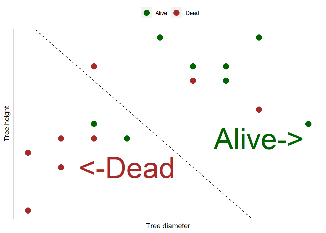
You can see that the model does a fairly good job of categorizing the trees as alive or dead. But there are three dead trees that were predicted to be alive. Plus, two alive trees were predicted to be dead.
- On paper or in R, create a small table that displays the confusion matrix for these observations and predictions. Label the true positive, false negative, false positive, and true negative values.
- Determine the accuracy of this model.
- The precision of a classification model measures the proportion of positive classifications that are correct. It is calculated as the number of true positive predictions divided by the total number of positive predictions (true and false). Calculate the precision of this model.
- The sensitivity (or recall) of a classification model measures the proportion of correct positives that were identified correctly. It is calculated as the number of true positive predictions divided by the total number of true positive and true negative predictions. Calculate the sensitivity of this model.
12.3 Modeling more than two responses
12.3.1 Multinomial logistic regression
There are many applications in natural resources when there is a binary response. But many other cases involve situations when there are three or more responses. In this case, a multinomial logistic regression can be performed when the response variable contains three or more categories that are not ordered. For example, a multinomial logistic regression can be performed to predict the nesting locations for a data set of bird species based on their physiological characteristics. These response variables could include trees, shrubs, the ground, or cliff and other high open areas.
Multinomial models are similarly fit using maximum likelihood techniques with a multinomial distribution. As the number of responses increases, the multinomial model becomes more complex. In R, the nnet package is useful for fitting multinomial logistic regression models. The package was created for designing neural networks, a tool used widely in machine learning (Venables and Ripley 2002):
install.packages("nnet")

library(nnet)
To see how logit regression models are fit to data with more than two responses, we will use data collected from a survey of over 300 private forest landowners in Minnesota, USA (UMN Extension Forestry 2021). The survey conducted an educational program needs assessment for this audience, inquiring about topics that participants are interested in learning about and future educational needs. Specifically, we may be interested in how differences in the ages of learners within this audience influence their preferred formats for learning about new educational opportunities and their comfort in virtual learning.

FIGURE 12.2: Forest landowners take part in an educational program. Photo by the author.
One question in the needs assessment inquired about the preferred format to learn about upcoming educational programs offered through the university. Landowners chose from the options of email, printed newsletter, social media, or website or blog. The data were collected across a range of four age groups:
m1.table## method
## age Email Printed newsletter Social media Website or blog
## 18-34 8 0 0 1
## 35-54 38 2 0 5
## 55-69 91 7 0 2
## 70 or over 43 10 1 0You will note that most landowners preferred email as a format, with fewer responses in the other categories. We seek to determine the preferred format based on age group because the response variable is not ordered and there are three or more categories. The multinom() function from the nnet package fits multinomial logistic regressions in a format similar to logistic regression. Again, specifying weights = Freq indicates to use the number of observations contained in the m1.table contingency table:
multi.learn <- multinom(method ~ age, weights = Freq, data = m1.table)## # weights: 20 (12 variable)
## initial value 288.349227
## iter 10 value 104.896727
## iter 20 value 92.578146
## iter 30 value 92.467996
## iter 40 value 92.448798
## iter 50 value 92.446478
## final value 92.446474
## convergedsummary(multi.learn)## Call:
## multinom(formula = method ~ age, data = m1.table, weights = Freq)
##
## Coefficients:
## (Intercept) age35-54 age55-69 age70 or over
## Printed newsletter -16.153156 13.20863573 13.588153 14.694491
## Social media -11.222075 -5.36141505 -11.896637 7.460595
## Website or blog -2.079573 0.05147451 -1.738202 -17.915025
##
## Std. Errors:
## (Intercept) age35-54 age55-69 age70 or over
## Printed newsletter 0.2240912 0.5598176 0.35657182 3.344345e-01
## Social media 96.6680976 654.5700991 0.05515755 9.667339e+01
## Website or blog 1.0607205 1.1625120 1.27911905 8.284796e-06
##
## Residual Deviance: 184.8929
## AIC: 208.8929The output reports the odds of selecting one of the preferred learning formats as a reference scenario (in this case, email). To decipher the output, the coefficients and standard errors for the numbers in the Printed newsletter row compare models determining the probability of preferring printed newsletters as a method compared to email. Values in other rows similarly compare different preferred methods relative to the reference email format. As an example, the log odds of preferring a printed newsletter compared to an email will increase by 14.69 if comparing those in the 18–34 to the 70 years or over age group.
Similar to logistic regression, you can exponentiate the coefficients in a multinomial logistic regression to determine the odds ratios:
exp(coef(multi.learn))## (Intercept) age35-54 age55-69
## Printed newsletter 9.655467e-08 5.450516e+05 7.966356e+05
## Social media 1.337564e-05 4.694259e-03 6.813277e-06
## Website or blog 1.249836e-01 1.052822e+00 1.758363e-01
## age70 or over
## Printed newsletter 2.408442e+06
## Social media 1.738182e+03
## Website or blog 1.658072e-08The predict() function can be used estimate multinomial probabilities. We will create a simple data set named age containing the four age groups, then bind it to a data set of predicted values containing the probabilities determined from the multi.learn object. We will then apply the pivot_longer() function to create a tidy data set containing three variables: age group, learning format, and probability.
age <- tibble(age = c("18-34", "35-54", "55-69", "70 or over"))

pred_multi <- cbind(age, predict(multi.learn,
                                 newdata = age,
                                 type = "probs"))

pred_multi_long <- pred_multi %>%
  pivot_longer(!age, names_to = "Format", values_to = "Prob")
We can plot the data to visualize the trends across age groups and the preferred format of learning about educational programs. A bar graph that is dodged by preferred format highlights these trends:
ggplot(pred_multi_long, aes(x = age, y = Prob, fill = Format)) +
geom_bar(stat = "identity", position = "dodge") 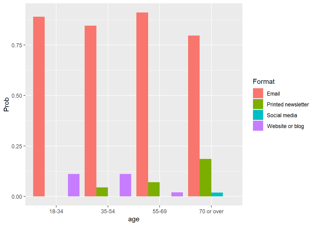
Here we can see the greater probability of older participants preferring printed newsletters as a format for learning about new programs. While younger audiences favor email heavily, older individuals have a lower preference for email as a medium.
DATA ANALYSIS TIP: Oftentimes it may be appropriate to “dichotomize” a multinomial variable into a binary one so that a simpler logistic regression analysis can be performed. For example, we could turn the learning format method variable into a binary one by labeling the formats as print (e.g., the print newsletter responses) or online (e.g., the email, social media, and website/blog responses). Then, we could perform logistic regression on this binary variable. Use caution with this approach, as you may lose important insights from specific groups when you combine and code them into different categories.
12.3.2 Ordinal regression
There may be other cases when there are three or more responses and there is an ordered relationship between the response variables. If a categorical variable is ordinal it indicates that the order of values is important, but the difference between each order cannot be quantified. A few examples in natural resources include:
- A survey provides a statement to participants and asks them to evaluate it on a five-point scale (e.g., a Likert (1932) scale) consisting of the responses strongly disagree, disagree, neither agree nor disagree, agree, or strongly agree.
- Pieces of downed woody debris are measured for their decay class (Harmon et al. 1986), a somewhat subjective measure of the reduction in volume, biomass, carbon, and density of dead wood, typically labeled from one (freshly fallen) through five (advanced decomposition).
- The production of leaves following herbicide applications on bald cypress trees measured from none to severe malformation (Sartain and Mudge 2018).
In these cases, ordinal regression, also termed cumulative logit modeling, can be performed when the response variable contains three or more categories that are ordered. In R, the MASS package introduced by Venables and Ripley (2002) is useful for fitting ordinal regression models:
install.packages("MASS")

library(MASS)
As an example, a different question in the forestry programming needs assessment asked respondents about their comfort in participating in online learning. This was essential information to be aware of during the COVID-19 pandemic when the majority of education occurred in an online virtual environment. Respondents were provided the statement “I feel comfortable participating in online learning” and were asked to choose from the options of “Always,” “Most of the time,” or “Never.” These responses can be considered an ordinal response because they reflect a decreasing comfort in online learning.
The data were summarized across the four age groups:
m2.table## comfort
## age Always Most of the time Never
## 18-34 11 0 0
## 35-54 41 7 2
## 55-69 87 23 3
## 70 or over 36 28 6Most respondents were comfortable with learning in an online environment at least most of the time, however, some individuals in older age groups indicated they were never comfortable with online learning. (As an aside, this was an interesting finding given that the needs assessment survey was an online one. Hence, the true number of individuals that are not comfortable with online learning is likely underestimated.)
In ordinal regression, the log odds of being less than or equal to a chosen category can be defined as:
\[log\frac{P(y\le j)}{P(y> j)}\]
where \(y\) is an ordered response and \(j\) is the number of responses. Given the nature of the ordered variable, we will model comfort as the response variable using the polr() function from the MASS package, which indicates probit or ordered logistic regression. We follow the general approach as used in multinomial logistic regression when applying it to the m2.table contingency table:
ord.learn <- polr(comfort ~ age, weights = Freq, data = m2.table)
summary(ord.learn)
## Call:
## polr(formula = comfort ~ age, data = m2.table, weights = Freq)
##
## Coefficients:
## Value Std. Error t value
## age35-54 15.71 0.2875 54.63
## age55-69 15.99 0.1991 80.29
## age70 or over 17.13 0.2057 83.28
##
## Intercepts:
## Value Std. Error t value
## Always|Most of the time 17.2017 0.1231 139.7747
## Most of the time|Never 19.4413 0.3095 62.8076
##
## Residual Deviance: 326.5716
## AIC: 336.5716The output provides the coefficients associated with each age group in addition to the intercept values. The residual deviance and AIC values allow us to compare the quality of the models to others. Similarly, the predict() function can be run on an ordinal regression object:
pred_ord <- cbind(age, predict(ord.learn,
                               newdata = age,
                               type = "probs"))

pred_ord_long <- pred_ord %>%
  pivot_longer(!age, names_to = "Comfort", values_to = "Prob")
We can plot the predictions to visualize the trends across age groups and participant comfort in online learning:
ggplot(pred_ord_long, aes(x = age, y = Prob, fill = Comfort)) +
geom_bar(stat = "identity", position = "dodge") 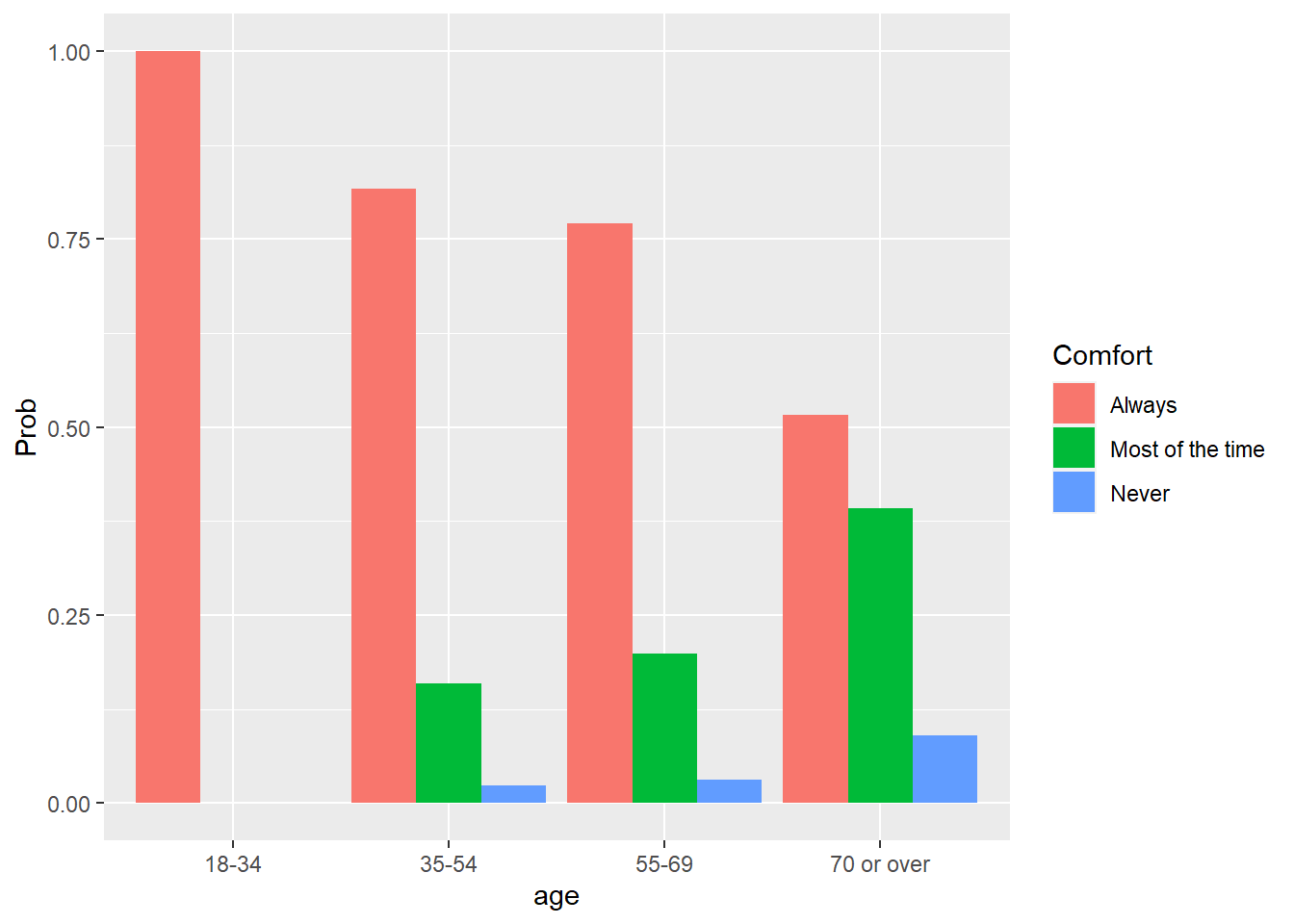
We see a greater probability of younger participants being comfortable with online learning, while older participants have a greater likelihood of stating they are comfortable with online learning “most of the time” or “never.” Similar to multinomial logistic regression, you can exponentiate the coefficients in an ordinal regression to determine the odds ratios.
12.3.3 Exercises
12.5 After investigating the fish data set from the stats4nr package, you suspect that you might be able to correctly identify a species of fish based on only a few key measurements. Perform the following analyses:
- Create a scatter plot of
WidthandLength1and color each point to correspond to one of the seven different fish species. - Using the
multinom()function from the nnet package, create a multinomial logistic regression model that predicts fish species based onWidthandLength1. - Use the model to predict the fish species from the data set named new.fish, containing various fish measurements. HINT: add
type = "class"within thepredict()function obtain the name of the fish species:
new.fish <- tibble(Width = c(10, 10, 12, 15, 20),
                   Length1 = c(10, 40, 32, 22, 30))
12.6 In question 12.3, we created a binary variable that categorized a cedar elm’s crown class code (CROWN_CLASS_CD) as either being intermediate or suppressed, or something else. We can actually consider the CROWN_CLASS_CD variable in the elm data set to be an ordinal one because trees that receive the most sunlight are categorized as a 1 (open-grown trees) and trees that receive the least sunlight are categorized as a 5 (suppressed trees).
- Perform an ordinal regression predicting
CROWN_CLASS_CDusingDIAandHTwith thepolr()function from the MASS package. TheCROWN_CLASS_CDis stored as a numeric variable in the data, so remember to convert it to a factor level prior to modeling. - Use the model to predict the probabilities of a tree being in each of the crown class codes from the data set named new.elm, containing various measurements of cedar elm trees. Which tree (i.e., its height and diameter) would have the greatest probability of being open grown? Which tree would have the greatest probability of being suppressed?
new.elm <- tibble(DIA = c(5, 10, 15, 20, 25, 30),
                  HT = c(20, 25, 30, 35, 40, 50))
12.4 Summary
Logistic regression has a number of applications in natural resources and is a useful tool when the response variable of interest and is categorical. Depending on the nature of the categorical response variable, the following provides a sample of which techniques and functions to use when fitting these models in R:
- Logistic regression is appropriate when the response variable is binary. Use the
glm()function available in base R. - Multinomial regression is appropriate when there are three or more categories. Use the
multinom()function from the nnet package. - Ordinal regression is appropriate when there are three or more categories that are ordered in their design. Use the
polr()function from the MASS package.
All of these functions are able to perform logistic regression procedures on a “tidy” data set of observations, where one row represents one observation, or a contingency table where categorical responses are summarized in a compact form. While most standard output in R and other statistical software programs provide coefficients in terms of log odds, exponentiating these values provides odds ratios which are more easily interpreted. Understanding both the confusion matrix and its accuracy values provides tremendous insight into the performance of logistic regression models, particularly when applied to data not used in model fitting. When comparing different models and the variables used in them, goodness of fit measures such as AIC work well in the evaluation process.
12.5 References
Harmon, M.E., J.F. Franklin, F.J. Swanson, P. Sollins, S.V. Gregory, J.D. Lattin, N.H. Anderson, S.P. Cline, N.G. Aumen, J.R. Sedell, G.W. Lienkaemper, K. Cromack, and K.W. Cummins. 1986. Ecology of coarse woody debris in temperate ecosystems. Advances in Ecological Research 15: 133-–302.
Likert, R. 1932. A technique for the measurement of attitudes. Archives of Psychology 140: 1-–55.
Reinhardt, J., M.B. Russell, W. Lazarus, M. Chandler, and S. Senay. 2019. Status of invasive plants and management techniques in Minnesota: results from a 2018 survey. University of Minnesota. Retrieved from the University of Minnesota Digital Conservancy. Available at: https://hdl.handle.net/11299/216295.
Saha, S., C. Kuehne, and J. Bauhus. 2017. Lessons learned from oak cluster planting trials in central Europe. Canadian Journal of Forest Research 47: 139–148.
Sartain, B.T., and C.R. Mudge. 2018. Effect of winter herbicide applications on bald cypress (Taxodium distichum) and giant salvinia (Salvinia molesta). Invasive Plant Science and Management 11: 136–142.
University of Minnesota Extension Forestry. 2021. Educational needs assessment of tree and woodland programs in Minnesota: results from a 2020 study. Retrieved from the University of Minnesota Digital Conservancy. Available at: https://hdl.handle.net/11299/218206
Venables, W. N., and B.D. Ripley. 2002. Modern applied statistics with S. Fourth edition. Springer, New York.