Chapter 14 Linear mixed models

14.1 Introduction

Mixed models have emerged as one of the go-to regression techniques in natural resource applications. This is attributed to several reasons and primarily relates to the nested structure of natural resources data, either in a spatial or temporal context. First, technicians may collect information on experimental units that are close to one another in space or time. Second, oftentimes the same experimental units (e.g., the identical plant of animal) are measured again following their initial measurement. Third, mixed models can account for hierarchy within data. As an example, forest plots are often collected within stands, stands are located within ownerships, and a collection of ownerships comprise a landscape. Finally, mixed models allow the inclusion of both fixed and random effects. Fixed effects can be considered population-averaged values and are similar to the parameters found in “traditional” regression techniques like ordinary least squares. Random effects can be determined for each parameter, typically for each hierarchical level in a data set.

This chapter will discuss the theory and application of linear mixed models. Importantly, we’ll learn how mixed models differ from ordinary least squares and other regression techniques, how to fit mixed models in R, and how to make predictions using mixed models in new applications.

14.2 Comparing ordinary least squares and mixed effects models

Recall back to simple linear regression where we used the concepts of least squares to minimize the residual sums of squares. This resulted in values for \(\beta_0\) and \(\beta_1\) that we considered constant or “fixed” (with some standard error associated with them).

\[Y = \beta_0 + \beta_1X+\varepsilon\]

The intercept (\(\beta_0\)) and slope (\(\beta_1\)) in simple linear regression will be chosen so that the residual sum of squares is as small as possible. For the same model in a mixed modeling framework, \(\beta_0\) and \(\beta_1\) are considered fixed effects (also known as the population-averaged values) and \(b_i\) is a random effect for subject \(i\). The random effect can be thought of as each subject’s deviation from the fixed intercept parameter. The key assumption about \(b_i\) is that it is independent, identically and normally distributed with a mean of zero and associated variance. For example, if we let the intercept be a random effect, it takes the form:

\[Y = \beta_0 + b_i + \beta_1X+\varepsilon\]

In this model, predictions would vary depending on each subject’s random intercept term, but slopes would be the same:

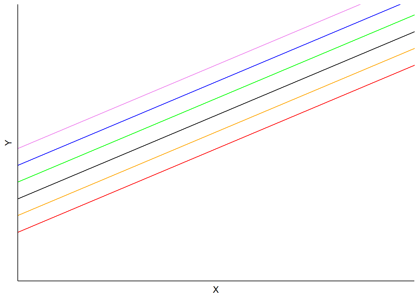
FIGURE 14.1: Example mixed model with random intercepts but identical slopes.

In another case, we can let the slope be a random effect, taking the form:

\[Y=\beta_0+(\beta_1+b_i)X+\varepsilon\]

In this model, the \(b_i\) is a random effect for subject \(i\) applied to the slope. Predictions would vary depending on each subject’s random slope term, but the intercept would be the same:

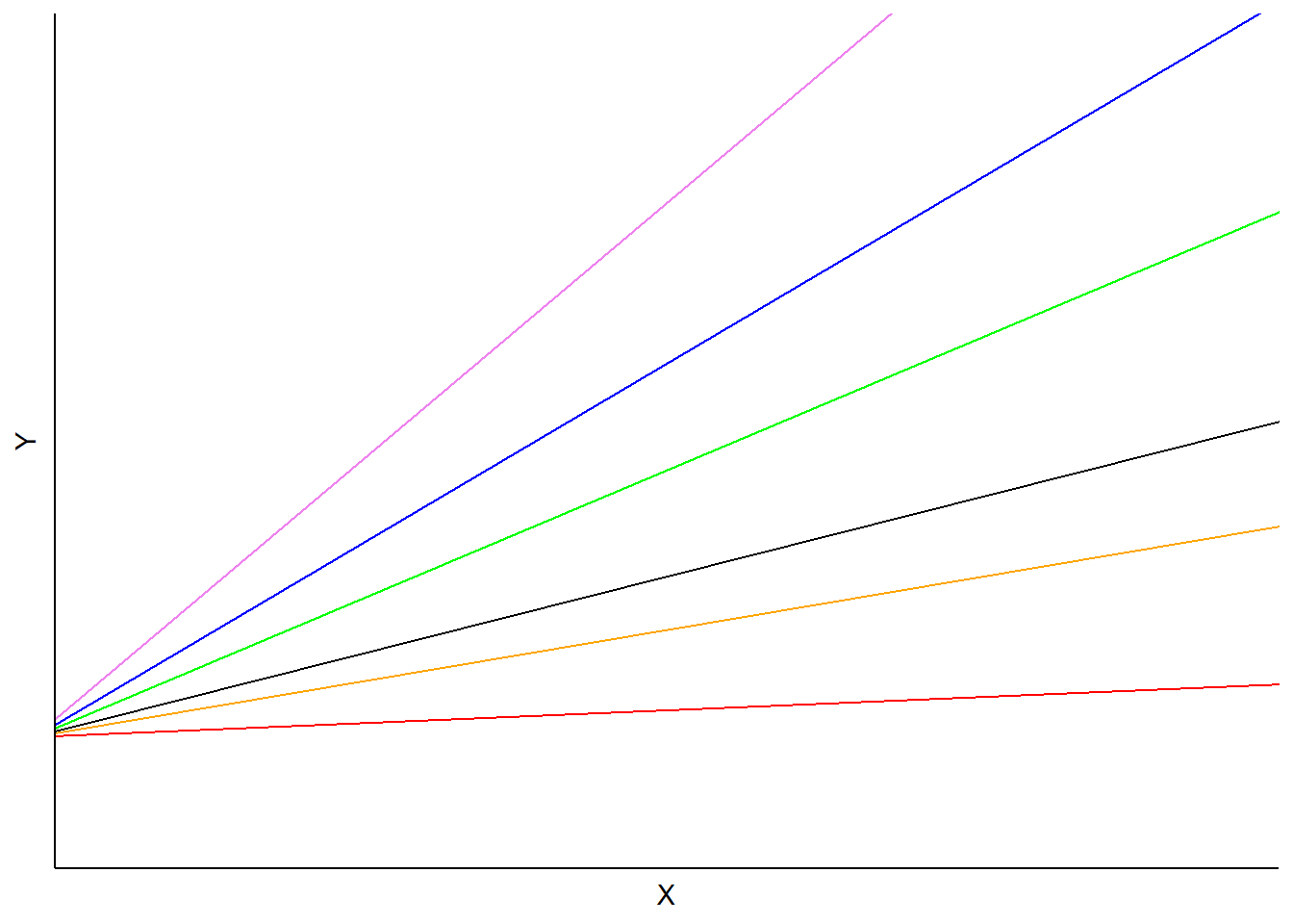
FIGURE 14.2: Example mixed model with random slopes but identical intercepts.

One could also specify a random effect term on both the intercept and slope. This model form would be:

\[Y=(\beta_0+a_i)+(\beta_1+b_i)X+\epsilon)\]

In this model, \(a_i\) and \(b_i\) are random effects for subject \(i\) applied to the intercept and slope, respectively. Predictions would vary depending on each subject’s slope and intercept terms:

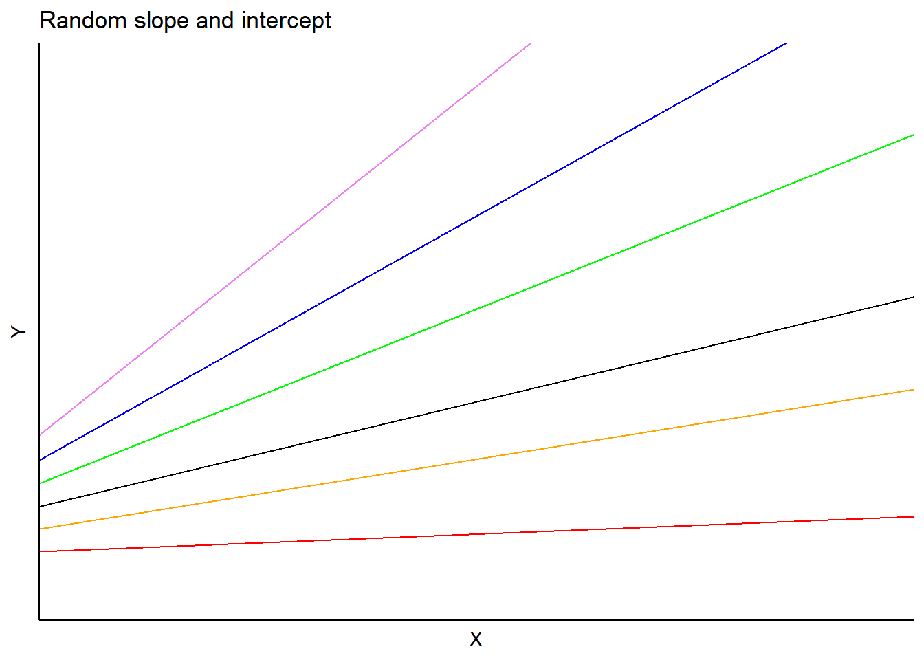
FIGURE 14.3: Example mixed model with random intercept and slopes terms.

One of the most popular applications of mixed models is to account for the nested or hierarchical structure of data. As an example, measurement plots within a forest are identified in forest resource assessments and measured to collect information of the status, size, and health of trees. These measurement plots are nested within forest stands, or areas of trees a similar size and age.

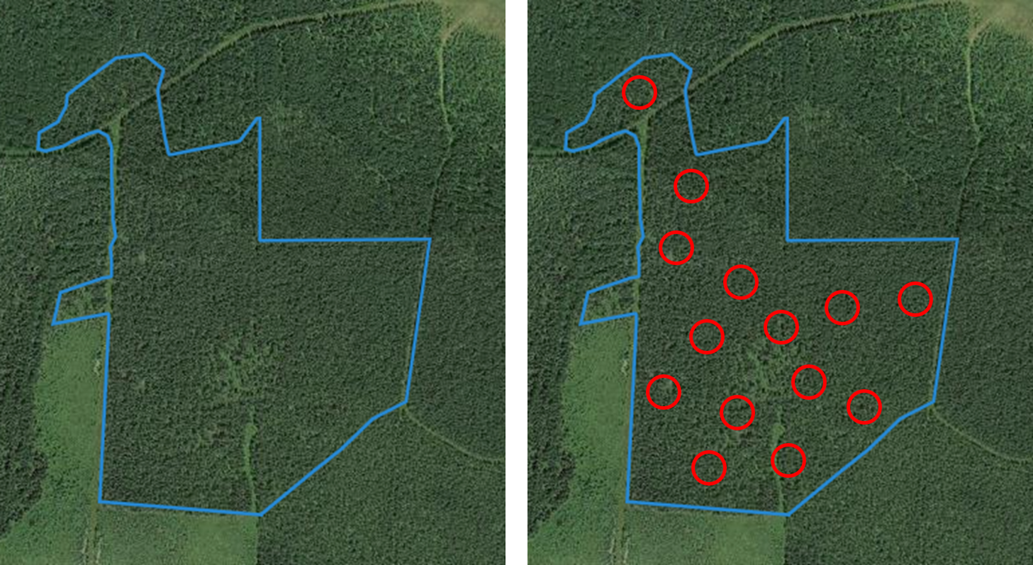
FIGURE 14.4: Forest stand (left) with measurement plots located throughout stand (right), showing nested design of data collection. Image: Ella Gray.

Consider a random effect term applied to the intercept. By nesting subject \(j\) within subject \(i\) (e.g., measurement plots nested withing stands), this model form would be:

\[Y = (\beta_0+b_i+b_{ij})+\beta_1X+\epsilon\]

In this model, \(b_i\) is the random effect for subject \(i\) and \(b_{ij}\) is the random effect for subject \(j\) nested in subject \(i\). In the forest plot example, we would obtain a set of random effects for each forest stand \(i\) and a set of random effects for each measurement plot nested within each stand \(ij\). Hence, predictions would result in two sets of random effects for each intercept (with identical slopes). Consider an example application with three stands and four plots located within those stands.

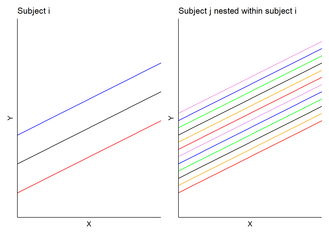
FIGURE 14.5: Example mixed model with random intercept terms applied to a nested design.

Even for a mixed model that uses one or only a few predictors, there are many choices for specifying which parameters should be random. To quantify this, you can fit several models with random effects applied to different parameters. After fitting models, you can evaluate them by assessing the quality of each model using metrics such as the Akaike information criterion (AIC) or a likelihood ratio test.

Another valid question is to ask whether mixed models are needed for your analysis. For example, a simple linear regression model fit with ordinary least squares may do. To examine this, fit a model with and without random effects. The various model forms can be evaluated with AIC or a likelihood ratio test. Lower AIC values for mixed model forms indicate that random effects are useful in the predictions.

14.2.1 Exercises

14.1 Many applications of mixed models are compared to those fit with ordinary least squares. Using the redpine data set from the stats4nr package, we are interested in predicting a tree’s height (HT) based on its diameter at breast height (DBH). Data are from 450 red pine (Pinus resinosa) observations made at the Cloquet Forestry Center in Cloquet, Minnesota in 2014 with DBH measured in inches and HT measured in feet.

1. Write code using the ggplot() function that produces a scatter plot of red pine diameter and height. Add a linear regression line to the plot.
2. Find the Pearson correlation coefficient between tree height (HT) and diameter at breast height (DBH).
3. Fit a regression equation using ordinary least squares predicting tree height based on its diameter.
4. Use the AIC() function to determine the Akaike information criterion of the fitted model.

14.3 Linear mixed models in R

Two popular R packages for performing mixed models in R are lme4 (for linear models) and nlme (for linear and nonlinear models). To learn more about the theory behind mixed models, Pinheiro and Bates (2000) and Zuur et al. (2009) are excellent sources.

14.3.1 Case study: Predicting tree height with mixed models

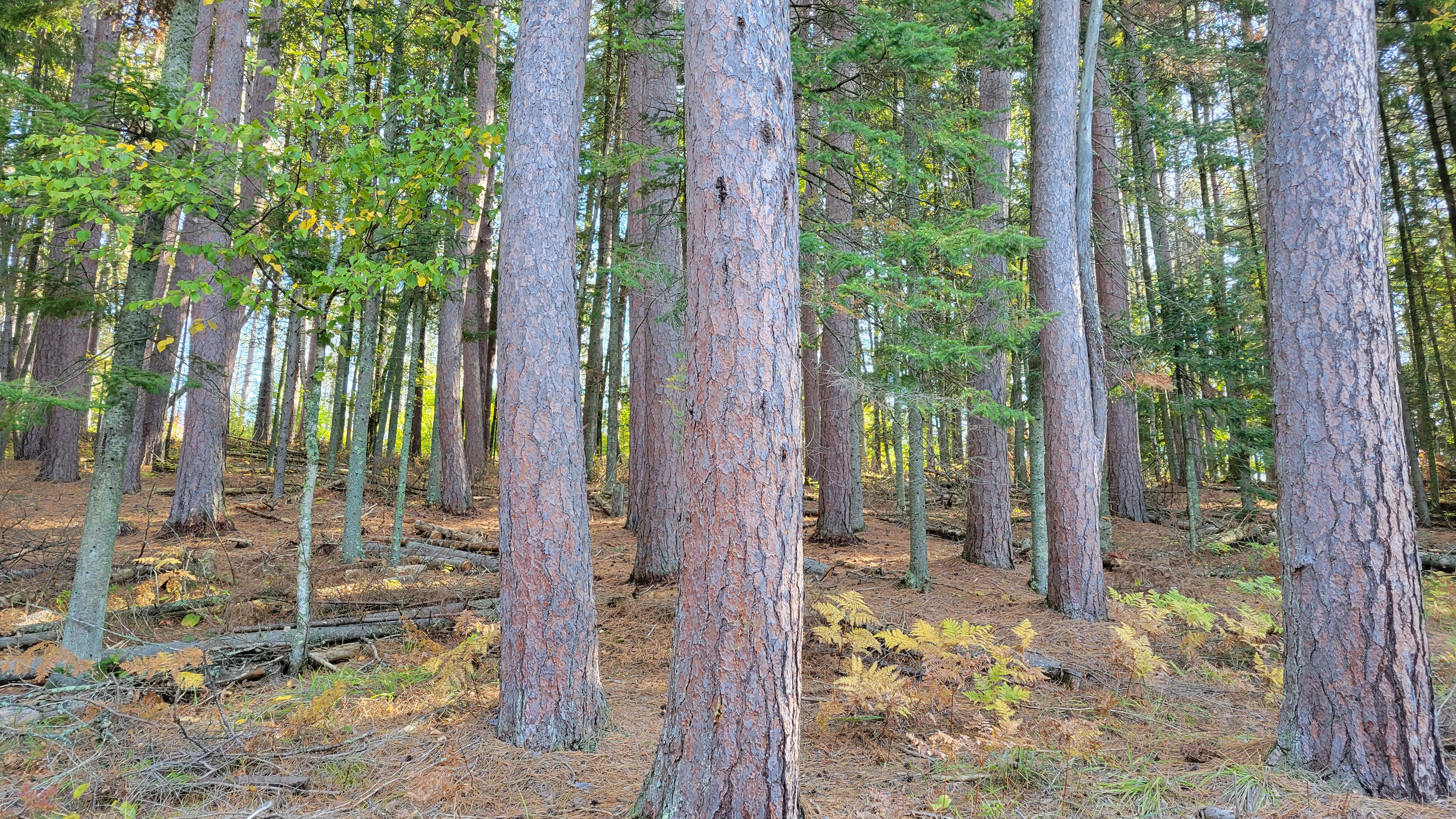
FIGURE 14.6: A stand of red pine trees in northern Minnesota, USA. Image by the author.

We seek to build upon the analysis of question 14.1 by predicting the height of red pine trees based on their diameter. Data were collected from various forest cover types (CoverType) and forest inventory plots (PlotNum) across the forest: The redpine data set from the stats4nr package contain the data:

library(stats4nr)

head(redpine)

## # A tibble: 6 x 5
##   PlotNum CoverType TreeNum   DBH    HT
##     <dbl> <chr>       <dbl> <dbl> <dbl>
## 1       5 Red pine       46  13      51
## 2       5 Red pine       50   8.3    54
## 3       5 Red pine       54   8.2    48
## 4       5 Red pine       56  11.8    55
## 5       5 Red pine       63   9      54
## 6       5 Red pine       71  12.5    46

14.3.1.1 Random effects on intercept

We can expand a simple linear regression to a mixed model by incorporating the forest cover type from where a tree resides as a random effect. Cover types are assigned in the field based on the dominant species occurring in a plot, hence, we might have reason to believe that variability may be observed as one transitions from one cover type to the next. In the red pine data, the n_distinct() function indicates there are 13 different cover types on the property:

n_distinct(redpine$CoverType)

## [1] 13

We can see that while most of the red pine trees are found in the red pine cover type, the species is also found in the other 12 cover types, although less abundant:

ggplot(redpine, aes(DBH, HT)) +
  geom_point() +
  facet_wrap(~CoverType, ncol = 4) +
  labs(x = "Diameter at breast height (inches)",
       y = "Height (feet)")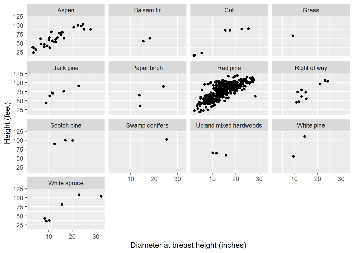 

FIGURE 14.7: The relationship between tree height and diameter in 13 different cover types in Cloquet, MN.

The lme4 package in R can be used to fit linear mixed models for fixed and random effects. We will use it to fit three linear mixed models that specify random effects on different parameters:

install.packages("lme4")
library(lme4)

The lmer() function is the mixed model equivalent of lm() and parameter estimates are fit using maximum likelihood. To specify the cover type as a random effect on the intercept, we write + (1 | CoverType) after specifying the independent variable DBH:

redpine.lme <- lmer(HT ~ DBH + (1 | CoverType),
             data = redpine)
summary(redpine.lme)

## Linear mixed model fit by REML ['lmerMod']
## Formula: HT ~ DBH + (1 | CoverType)
##    Data: redpine
## 
## REML criterion at convergence: 3652
## 
## Scaled residuals: 
##     Min      1Q  Median      3Q     Max 
## -4.1165 -0.6923 -0.0591  0.6087  3.0488 
## 
## Random effects:
##  Groups    Name        Variance Std.Dev.
##  CoverType (Intercept)  52.24    7.228  
##  Residual              191.14   13.825  
## Number of obs: 450, groups:  CoverType, 13
## 
## Fixed effects:
##             Estimate Std. Error t value
## (Intercept)  25.8867     3.2321   8.009
## DBH           3.0585     0.1169  26.169
## 
## Correlation of Fixed Effects:
##     (Intr)
## DBH -0.537

The lmer() output contains similar-looking output compared to lm(). We can see from the output that the values for the fixed effects \(\beta_0\) and \(\beta_1\) are 25.8867 and 3.0585, respectively. The Random effects section contains details on the variance of the CoverType random effect and the residuals. Note the residual standard error of 13.825 feet, which can be compared to the value 14.31 obtained through fitting a model with ordinary least squares for question 14.1.

The ranef() function extracts the random effect terms from a mixed model. In this model, we can obtain the 13 random effects for each cover type:

ranef(redpine.lme)

## $CoverType
##                        (Intercept)
## Aspen                   -2.4313290
## Balsam fir              -6.4569721
## Cut                     -5.3398733
## Grass                    3.2321996
## Jack pine                1.1099090
## Paper birch             -7.0258594
## Red pine                 6.4705981
## Right of way             0.7999610
## Scotch pine              8.9566777
## Swamp conifers          -0.3374007
## Upland mixed hardwoods  -0.9416721
## White pine               6.9294464
## White spruce            -4.9656851
## 
## with conditional variances for "CoverType"

As a visual, the HT-DBH models with varying random intercepts will show a different regression line for each cover type. We will specify a predict() statement within geom_line() to visualize the predictions.

ggplot(redpine, aes(DBH, HT)) +
   geom_point(size = 0.2) +
   geom_line(aes(y = predict(redpine.lme), 
                 group = CoverType, 
                 color = CoverType)) +
   labs(x = "Diameter at breast height (inches)",
        y = "Height (feet)")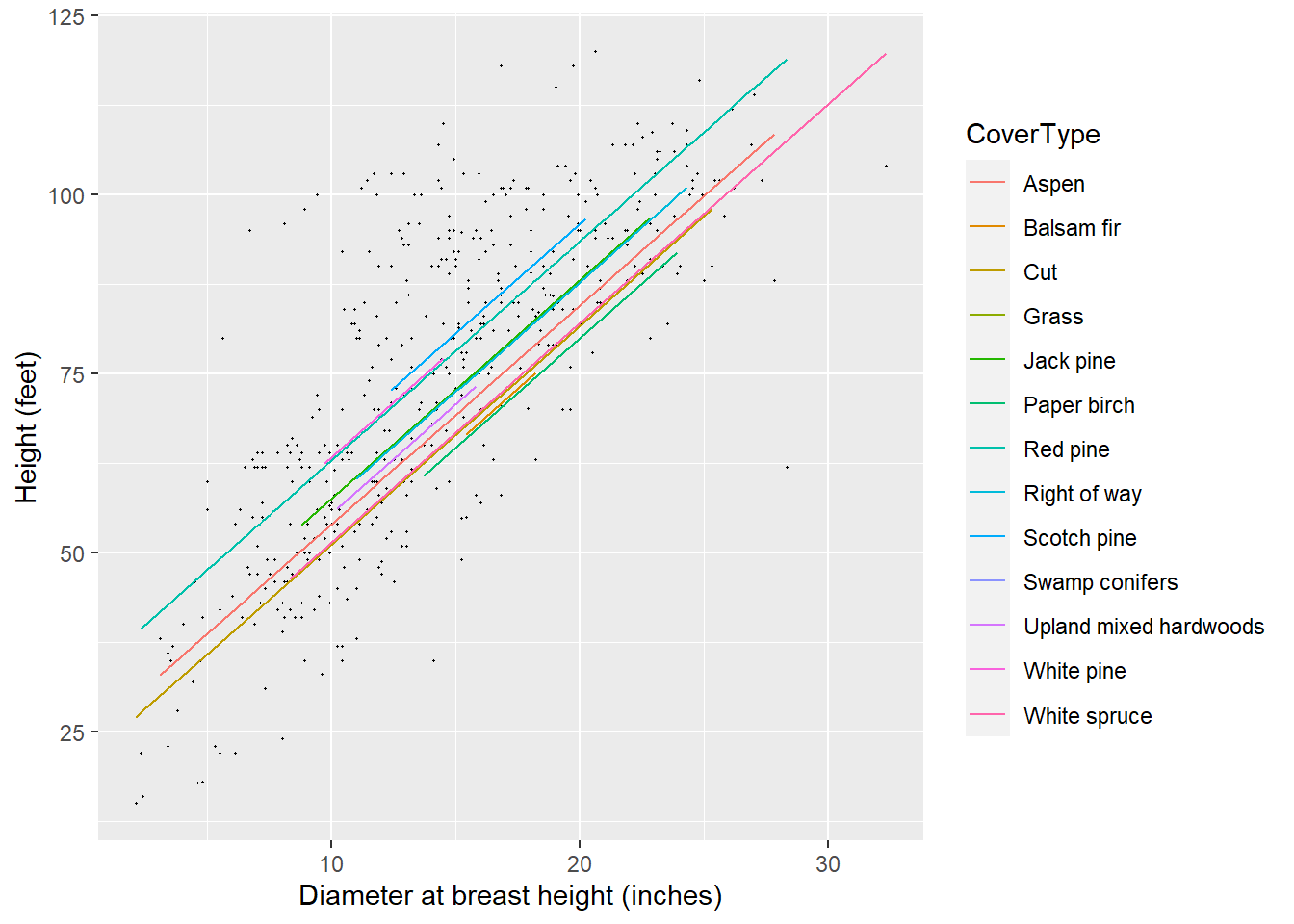

FIGURE 14.8: The height-diameter regression lines after fitting forest cover type as a random effect to predict red pine tree heights in Cloquet, MN.

Note that the lines have the same slope yet different intercepts, as depicted in the random effect term applied to \(\beta_0\). You will notice that some predictions do not extend far through the x-axis, a reflection of the small sample size for red pine trees found in some cover types.

For the same tree diameter, the mixed model predictions indicate that trees growing in the Scotch pine (Pinus sylvestris) and red pine cover types would be tallest. Trees growing in the balsam fir and paper birch cover types would be shortest. Oftentimes with natural resources data, the distribution and magnitude of random effects can help to reinforce biological findings. For example, a wise forester may tell you that “pine trees grow well where pine trees should be growing.” That is, taller red pine trees growing in pine cover types would be a likely outcome contrasted with red pine trees growing where fir and birch trees are better adapted.

14.3.1.2 Random effects on slope

An alternative mixed model could be specified by placing a random parameter on the slope term, which can potentially introduce model complexity. In the tree height example, we can specify (1 + DBH | CoverType) to place a random effect on the slope term for DBH:

redpine.lme2 <- lmer(HT ~ 1 + DBH + (1 + DBH | CoverType),
             data = redpine)
summary(redpine.lme2)

## Linear mixed model fit by REML ['lmerMod']
## Formula: HT ~ 1 + DBH + (1 + DBH | CoverType)
##    Data: redpine
## 
## REML criterion at convergence: 3651.7
## 
## Scaled residuals: 
##     Min      1Q  Median      3Q     Max 
## -4.0915 -0.6998 -0.0553  0.6024  3.0359 
## 
## Random effects:
##  Groups    Name        Variance  Std.Dev. Corr 
##  CoverType (Intercept)  78.74861  8.8740       
##            DBH           0.01029  0.1014  -1.00
##  Residual              190.92366 13.8175       
## Number of obs: 450, groups:  CoverType, 13
## 
## Fixed effects:
##             Estimate Std. Error t value
## (Intercept)  24.9363     3.7333   6.679
## DBH           3.1208     0.1235  25.269
## 
## Correlation of Fixed Effects:
##     (Intr)
## DBH -0.706
## optimizer (nloptwrap) convergence code: 0 (OK)
## boundary (singular) fit: see ?isSingular

You can see that the error message boundary (singular) fit: see ?isSingular is shown, indicating that the model is likely overfitted. We may be trying to do too much by specifying the random effects on the slope. Hence, for these data, we might forgo the inclusion of a random slope parameter and instead focus on random effects for the intercept.

14.3.1.3 Nested random effects on intercept

We can expand the mixed model by incorporating the measurement plot (PlotNum) nested within forest cover type (CoverType) as random effects in the prediction of tree height. In the red pine data, there are 124 plots nested within the 13 cover types found in the data:

n_distinct(redpine$PlotNum)

## [1] 124

It would be challenging to view scatter plots that show the height-diameter relationship for each plot, however, adding facet_wrap() to ggplot code can visualize important differences in these trends. For example, note the distributions of red pine heights and diameters in plots 24 and 102. For the same range in diameters for both trees, note the taller heights for those in plot 24:

redpine %>% 
   filter(PlotNum == c(24, 102)) %>% 
   ggplot(aes(DBH, HT)) +
  geom_point() +
  facet_wrap(~PlotNum) +
  labs(title = "Red pine at Cloquet Forestry Center",
       subtitle = "HT-DBH by plot number",
       x = "Diameter at breast height (inches)",
       y = "Height (feet)")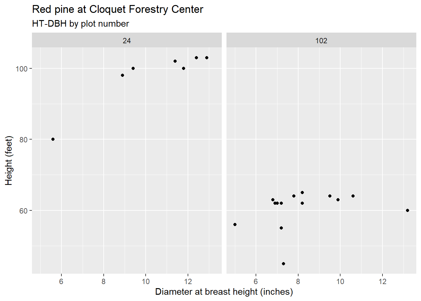

To specify nested random effects on the intercept (plot number nested within cover type), we can write (1 | CoverType/PlotNum) in the lmer() function:

redpine.lme3 <- lmer(HT ~ DBH + (1 | CoverType/PlotNum),
             data = redpine)
summary(redpine.lme3)

## Linear mixed model fit by REML ['lmerMod']
## Formula: HT ~ DBH + (1 | CoverType/PlotNum)
##    Data: redpine
## 
## REML criterion at convergence: 3413
## 
## Scaled residuals: 
##     Min      1Q  Median      3Q     Max 
## -3.8376 -0.4860  0.0388  0.5710  3.1585 
## 
## Random effects:
##  Groups            Name        Variance Std.Dev.
##  PlotNum:CoverType (Intercept) 123.63   11.119  
##  CoverType         (Intercept)  19.17    4.378  
##  Residual                       68.73    8.291  
## Number of obs: 450, groups:  PlotNum:CoverType, 124; CoverType, 13
## 
## Fixed effects:
##             Estimate Std. Error t value
## (Intercept)  30.5389     2.9080   10.50
## DBH           2.7111     0.1192   22.74
## 
## Correlation of Fixed Effects:
##     (Intr)
## DBH -0.621

In this model, the estimated values of \(\beta_0\) and \(\beta_1\) are 30.5389 and 2.7111, respectively. Note that these values are slightly different from previous model fits. In this model, we can obtain the 13 random effects for each cover type and 124 random effects for each plot nested within each cover type.

ranef.lme3 <- ranef(redpine.lme3)

A quantile-quantile plot indicates the random effects are generally normally distributed:

plot(ranef.lme3)

## $`PlotNum:CoverType`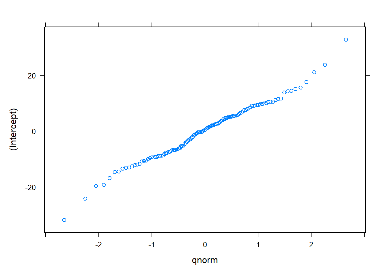

## 
## $CoverType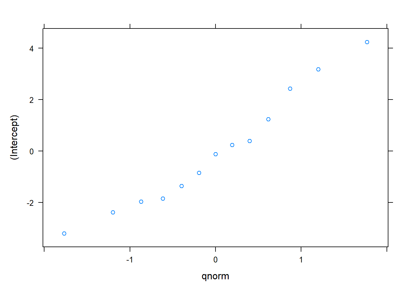

We can compare the AIC for each mixed model form fit with random effects applied to the intercept:

AIC(redpine.lme, redpine.lme3)

##              df      AIC
## redpine.lme   4 3659.952
## redpine.lme3  5 3422.994

Each model form, including the ordinary least squares model (from question 14.1) and linear mixed models is summarized in Table 1.

TABLE 14.1: Summary of ordinary least squares and linear mixed models fit with random effects applied to the intercept for the red pine data.

Model	Intercept	Slope	AIC
OLS	31.05	3.05	3676.1
Random = Cover Type	25.89	3.06	3660.0
Random = Cover Type/Plot	30.54	2.71	3423.0

Note that the AIC is lowest for the mixed model with the plot nested within cover type. While the emphasis here is on fitting linear mixed models, you may be interested in exploring the glmer() and nlmer() functions from lme4 for fitting generalized linear and nonlinear mixed models, respectively.

14.3.2 Exercises

14.2 Use the fish data set from the stats4nr package to answer the following questions.

1. Using ggplot(), make a scatter plot showing the weight of the fish (Weight; in grams) on the y-axis and the length from the nose to the beginning of the tail (Length1; in cm) on the x-axis. Color the observations for each of the seven species and add a stat_smooth() statement that displays a linear regression line for each species.
2. Fit a linear mixed model predicting Weight based on Length1 that incorporates Species as a random effect on the intercept.
3. Fit a similar linear mixed model predicting Weight based on Length1, but this time apply the random effect of Species on the slope term.
4. Compare the AIC values of the models in parts b and c. Which model may be preferred and why?

14.3 Use Loblolly, a built-in data set in R containing the height, age, and seed source of loblolly pine (Pinus taeda) trees, to answer the following questions.

1. Fit a linear mixed model predicting tree height (height; in meters) based on tree age (age; years) that incorporates seed source as a random effect on the intercept. Create a quantile-quantile plot to assess whether the random effects are normally distributed.
2. Ben Bolker created broom.mixed, an R package that extends what the broom package does to different kinds of model forms, including linear mixed models (Bolker 2021). Install and load the package, then use the augment() function to extract the fitted and residual values for the observations in Loblolly. Hint: consult section 8.6.2 where we do a similar activity with the broom package in an ordinary least squares regression.
3. Create a scatter plot of residual and fitted values using ggplot() and add a smoothed trend line. What do you notice about the model and how might it be remedied?

14.4 The lmerTest package in R provides additional output and functions that work with linear mixed models fit with lmer(). After installing and loading the package, explore its ranova() function. This function performs a likelihood ratio test that assesses the contribution of random effects in a linear mixed model. Apply the function to the models fit with random effects on the intercept from questions 14.2 (the fish data) and 14.3 (the loblolly pine data). What is the result of the likelihood ratio tests, that is, do the random effects contribute to the performance of the model?

14.4 Predictions and local calibration of mixed models

14.4.1 Predictions for observations used in model fitting

Mixed models are advantageous because of their inclusion of random effects that may account for the hierarchy of data. If you are interested in making predictions for observations used in the model fitting, you have two options:

• Use the fixed effects alone to make predictions. This is identical to setting the random effect terms equal to zero.
• Use the subject-specific random effects. In this approach, you create best linear unbiased predictions (BLUPs) to estimate random effects for linear mixed models.

As an example, consider we wish to make two sets of predictions for red pine heights using the model with a random effect for cover type applied to the intercept. Note that the coef() function applied to this model reveals the different intercepts for the 13 cover types with an identical slope:

coef(redpine.lme)

## $CoverType
##                        (Intercept)     DBH
## Aspen                     23.45539 3.05847
## Balsam fir                19.42975 3.05847
## Cut                       20.54684 3.05847
## Grass                     29.11892 3.05847
## Jack pine                 26.99663 3.05847
## Paper birch               18.86086 3.05847
## Red pine                  32.35732 3.05847
## Right of way              26.68668 3.05847
## Scotch pine               34.84340 3.05847
## Swamp conifers            25.54932 3.05847
## Upland mixed hardwoods    24.94505 3.05847
## White pine                32.81616 3.05847
## White spruce              20.92103 3.05847
## 
## attr(,"class")
## [1] "coef.mer"

We will make one set of predictions using the fixed effects only and another using the subject-specific random effects. In R, the predict() function makes model predictions from different model types. For predictions from models fit with the lmer() function, a minimum of three arguments are needed:

• First, specify the R object that stores the model (e.g., redpine.lme).
• Second, specify the data set in which to apply to the predictions. In our case, we will add a new column to the original redpine data set.
• Lastly, use the re.form statement to specify whether you want to make predictions using fixed effects only or predictions using subject-specific random effects (e.g., BLUPs). If re.form = NULL, predictions are made including all random effects. If re.form = NA, predictions are made using fixed effects only (equivalent to setting the random effects equal to zero).

We can apply these new predictions by creating new variables using mutate() in the redpine data set and printing the first 10 rows of data using the top_n() function:

redpine <- redpine %>% 
   mutate(HT_pred_fixed_re = predict(redpine.lme, 
                                     redpine, 
                                     re.form = NULL),
          HT_pred_fixed = predict(redpine.lme, 
                                  redpine, 
                                  re.form = NA))

redpine %>% 
   top_n(10)

## Selecting by HT_pred_fixed

## # A tibble: 10 x 7
##    PlotNum CoverType    TreeNum   DBH    HT HT_pred_fixed_re
##      <dbl> <chr>          <dbl> <dbl> <dbl>            <dbl>
##  1      40 White spruce       4  32.3   104             120.
##  2      41 Red pine           1  27.7   108             117.
##  3      45 Red pine          13  27.3   102             116.
##  4     208 Red pine           1  26.9   107             115.
##  5     236 Red pine           7  26.1   112             112.
##  6     275 Aspen              4  27.8    88             108.
##  7     306 Red pine          20  26.2   101             112.
##  8     316 Red pine          10  28.3    62             119.
##  9     320 Red pine           2  27     114             115.
## 10     340 Red pine           1  25.8    97             111.
## # ... with 1 more variable: HT_pred_fixed <dbl>

Note the differences in the predictions of heights based on the two approaches.

14.4.2 Predictions for observations not used in model fitting

For making predictions outside of the original data used in model fitting, there are several approaches. First, you can make predictions using fixed effects, only. This is the most common approach one would choose when applying a mixed model. As we’ll learn shortly, mixed models can be locally calibrated, however, a subsample of the response variable is needed and is not often available. Oftentimes, with natural resources data, we implement experiments to monitor outcomes that are not immediately observed, hence, local calibration is not possible and we must rely on fixed effects predictions.

If a subset of measurements of the response variable are available, a second approach involves local calibration to improve the precision of estimates. With data that are derived from diverse populations, such as a tree of a single species from a forest with 100 plant species, local calibration can better reflect local environmental conditions and microclimates. For example, Temesgen et al. (2008) observed that a locally calibrated mixed model predicting the height of Douglas-fir trees outperformed predictions using fixed effects only.

Local calibration can be conducted after taking a subsample of the response variable (e.g., the height of the tree) and determining the estimated BLUPs for the mixed model. The drawback of this approach is that new measurements need to be obtained for the variable you seek to predict. However, researchers have observed that using even a single observation to locally calibrate a mixed model leads to better precision in estimates (Trincado et al. 2007, Temesgen et al. 2008). An excellent worked example predicting tree height using local calibrations for a nonlinear model form can be found in VanderSchaaf (2012).

A final approach, which may see limited applications depending on the variable chosen for the random effect, involves using the estimated random effects from the model fit in the prediction of new observations. In our analysis of red pine tree heights, we could use the estimated random effects for cover type to make new predictions for tree heights found in that cover type. For example, Kuehne et al. (2020) observed that using random effects from a mixed model predicting tree diameter growth with species as a random effect outperformed a fixed effects model fit only to that species. In addition, making growth predictions by extracting the random effects was robust to account for tree growth of species with only a few observations. Using the lmer package, this would be equivalent to using the predict() function on a data set of new observations and specifying re.form = NULL.

This final approach has a few drawbacks in that you may have observations in a new data set from subjects that were not contained in the data set used in model fitting. For example, you may encounter a new species which you have not estimated a random effect for. The choice to use this approach would also depend on the variable chosen for the random effect in the model. For example, you might assume that tree species and cover type can be identified in future observations you might make, however, oftentimes random effects are specified to account for attributes that are less biologically meaningful. For example, unique values such as the measurement plot, blocking unit, or replication unit are often specified as random effects in natural resources studies. It is impractical to use the extracted values from these random effects and apply them to new observations. If this approach is not practical, consider making predictions using fixed effects only or locally calibrating.

14.4.3 Exercises

14.5 Recall the linear mixed model you created in question 14.2c that predicted fish weight based on its length with the random effect of species on the slope term. Answer the following questions using the fish data set.

1. Write code in R to predict Weight based on Length1 using fixed effects, only.
2. Write code in R to predict Weight based on Length1 using the estimated BLUPs that incorporate Species as the random effect.
3. Calculate the mean bias of each prediction of fish weights. Mean bias can be obtained by calculating the difference between each observation and its prediction and then averaging these values. Based on the calculations, on average which prediction approach would you prefer?

14.6 You have collected ten more observations on the ages of loblolly pine trees and wish to apply the linear mixed model you created in question 14.3 to predict their heights. The data were collected from three seed sources that were also measured in the data set used in model fitting:

TABLE 14.2: Ten new observations of loblolly pine tree ages from different seed sources.

Seed	age
305	7
305	9
305	15
321	5
321	6
321	19
327	4
327	12
327	22
327	24

1. Write code in R to make two predictions of loblolly pine tree heights using this new data set: one using fixed effects only and the other using the extracted random effects from the model you fit that incorporated Seed as the random effect.
2. Make a scatter plot of predicted tree heights (y-axis) along the range of tree ages (x-axis) for these 10 observations. Add a col = statement to your code in ggplot() to make two colors for each of the different kinds of model predictions. Explain the differences you observe in the predictions in a sentence or two.

14.5 Opportunities and limitations of mixed models

We have discussed many of the benefits of mixed models, including their ability to account for data collected in a hierarchical structure and to provide more precise predictions compared to regression using ordinary least squares. These reasons alone make them popular analytical techniques to use with natural resources data. Other potential applications of mixed models include using them to predict missing values. For example, mixed models can be fit to a data set and then locally calibrated to estimate missing values. Mixed models are also fitting to analyze experimental data with blocking and replicate effects in addition to studies that make repeated measurements on the same subjects over time (West et al. 2015).

Despite their popularity, there are drawbacks to the use and implementation of mixed models. While computational resources have expanded greatly in recent years, fitting mixed models remains computationally demanding in some settings. In particular with natural resources data, models fit to data sets with a large number of observations (e.g., greater than 100,000) with multiple variables can often fail to converge or encounter problems during the model fitting process. Random effects applied to slope terms often require more time and effort to converge compared to when random effects are applied to intercept.

Mixed models also suffer from the need to continually evaluate them with other regression techniques. Mixed models often need to be evaluated with other model forms, including comparisons with models fit with ordinary least squares and those with and without random effects. Mixed models also may need to be refit iteratively to determine which parameters should be specified as random in a model. While additional effort may be needed to decide whether or not mixed models are appropriate for your analysis, functions that provide useful metrics such as AIC and likelihood ratio tests can aid in the determination of the applicability of mixed models in your own work.

14.5.1 Exercises

14.7 While much of this chapter has presented mixed models in the context of regression, they can also be implemented to analyze experimental treatments, similar to analysis of variance. To see this in practice, install the MASS package and load the oats data set found within it. These data contain the yield of oats from a field trial with three oat varieties and four levels of nitrogen (manure) treatment. Type print(oats) and ?oats in R and investigate the data. Create a linear mixed model using the lmer() function that predicts oat yield with variety, nitrogen treatment, and their interaction as fixed effects. Specify the experimental block as a random effect on the intercept. Use the anova() function to print the results. What roadblocks do you encounter when looking to assess the significance of the variety and nitrogen treatments?

14.8 The nlme package performs linear and nonlinear mixed effects modeling. Investigate the package by typing ?nlme and perform the same linear mixed model as in question 14.7 using its lme() function. At a level of significance of \(\alpha = 0.05\), do the variety, nitrogen treatments, and their interaction influence oat yield?

14.9 The CO2 data set records the carbon dioxide uptake in different plant grasses subject to varying treatments. Type print(CO2) and ?CO2 in R and investigate the data. Say you are interested in creating a mixed model to predict uptake based on all of the other variables in the data. How would you specify your model and which parameters/variables would you consider fixed and random effects?

14.6 Summary

Natural resources data are fitting to analyze with mixed models because data are often nested and subjects are often measured repeatedly though time. Mixed models differ from traditional regression techniques such as ordinary least squares by including random effects terms that can be applied to different parameters within a fitted equation. The lme4 and nlme packages in R are some of the most popular ones for fitting and making inference with mixed models.

Making new predictions with mixed models presents several options for an analyst. If a subsample of the response variable is available, mixed models can be calibrated with local observations to result in a more precise estimate. More often, additional data is not practical to obtain, hence, predictions using mixed models can be made using only the fixed effects or population average values. The implementation and application of mixed models requires a thorough evaluation to determine whether or not random effects are needed, and if so, which parameters should be specified as random. The application of mixed models in natural resources can help to fill in missing data, analyze data from experimental trials, and account for the unique attributes of data collected in a longitudinal format.

14.7 References

Bolker, B. 2021. Introduction to broom.mixed. Available at: https://cran.r-project.org/web/packages/broom.mixed/vignettes/broom_mixed_intro.html

Kuehne, C., M.B. Russell, A.R. Weiskittel, and J.A. Kershaw. 2020. Comparing strategies for representing individual-tree secondary growth in mixed-species stands in the Acadian Forest region. Forest Ecology and Management 459: 117823.

Pinheiro, J.C., and D.M. Bates. 2000. Mixed-effects models in S and S-PLUS. Springer-Verlag, New York.

Temesgen, H., V.J. Monleon, and D.W. Hann. 2008. Analysis and comparison of nonlinear tree height prediction strategies for Douglas-fir forests. Canadian Journal of Forest Research 38: 553–565.

Trincado, G., C.L. VanderSchaaf, and H.E. Burkhart. 2007. Regional mixed-effects height-diameter models for loblolly pine (Pinus taeda L.) plantations. European Journal of Forest Research 126: 253–262.

VanderSchaaf, C.L. 2012. Mixed-effects height-diameter models for commercially and ecologically important conifers in Minnesota. Northern Journal Applied Forestry 29: 15–20.

West, B.T., K.B. Welch, and A.T. Galecki. 2015. Linear mixed models: a practical guide using statistical software, 2nd ed. Chapman and Hall/CRC, Boca Raton, FL. 440 pp.

Zuur, A., E.N. Ieno, N. Walker, A.A. Saveliev, and G.M. Smith. 2009. Mixed effects models and extensions in ecology with R. Springer-Verlag, New York. 574 pp.