Chapter 6 Inference for two-way tables
6.1 Introduction
If data are collected as counts with two outcomes and two groups (e.g., the presence/absence of a species in two different regions), we can perform hypothesis tests for proportions. What adds more complexity is when it is possible to have more than two outcomes or groups being tested against, e.g., the presence/absence of a species in four different regions. Count data are quantitative, and a categorical data analysis technique will allow us to properly analyze these data across groups.
Storing data in two-way tables will allow us to visualize these counts across groups in an efficient way. Two-way tables and their analysis are common when experimenting with survey data and categorical data in natural resources. The chi-squared test and the statistic it provides will measure how far the observed counts are from what we expect them to be, ultimately telling us about the association across groups. As a result of this, our hypothesis test will reflect whether or not we can say that the groups are independent from one another.
6.2 Data in two-way tables
Two-way tables can show a lot of information in a compact form. A lot of published data such as survey results are summarized in this format. As an example, we might ask citizens whether or not they approve of the performance of a political candidate (yes or no) by their political party (e.g., liberal or conservative).
A few characteristics of two-way tables are that they:
- describe two categorical variables,
- organize counts in rows and columns, and
- show the number of counts within each cell.
The rows of a two-way table are the values of one categorical variable, and the columns are the values of the other categorical variable. The count in any particular cell of the table equals the number of subjects who fall into that cell.
Consider an example with diseased ruffed grouse. In 2018, a multi-state effort examined the presence of West Nile virus in ruffed grouse populations across the US Lake States. The study concluded that while the West Nile virus was present in the region, grouse that were exposed to the virus could survive.
The total number of ruffed grouse sampled that showed antibodies consistent with West Nile virus is shown by creating the two-way table below. The matrix() function creates a table with three states and the number of grouse that tested positive or negative for the virus:
grouse <- matrix(c(185, 28, 239, 34, 167, 68), nrow = 3, byrow = T)
colnames(grouse) <- c("West Nile Negative", "West Nile Positive")
rownames(grouse) <- c("Michigan", "Minnesota", "Wisconsin")
grouse
## West Nile Negative West Nile Positive
## Michigan 185 28
## Minnesota 239 34
## Wisconsin 167 68We can see that Minnesota had the greatest number of negative West Nile cases (239) and Wisconsin had the greatest number of positive West Nile cases (68). Visualizing data in this two-way table will help us to set up and interpret the results of a chi-squared test.
It also might help to add a total column to grouse that calculates the total number of grouse for each state and negative/positive outcome. This can be accomplished with the addmargins() function:
addmargins(grouse)## West Nile Negative West Nile Positive Sum
## Michigan 185 28 213
## Minnesota 239 34 273
## Wisconsin 167 68 235
## Sum 591 130 721We can easily see that 721 total grouse were sampled across the three states and 130 of them tested positive for West Nile.
6.3 The chi-squared test for two-way tables
The goal of a chi-squared test is to test the null hypothesis (\(H_0\)) that there is no relationship between the two categorical variables. In the grouse example, \(H_0\) would be that there is no relationship between positive West Nile cases and the state where they were sampled.
To perform a chi-squared test, we compare the actual counts (from the sample data) with expected counts (those expected when there is no relationship between the two variables). The expected count in any cell of a two-way table when \(H_0\) is true is:
\[\text{expected count} = \frac{\text{row total} \cdot \text{column total}}{n}\]
With \(r\) rows and \(c\) columns in a two-way table, there are \(r \cdot c\) possible cells. The chi-squared statistic, denoted \(\chi^2\), measures how far the actual counts are from the expected counts. In this case, “actual” counts are from the sample data and “expected” counts represent the expected count for the same cell. After summing all values in each \(r \cdot c\) cell in the table, the result is the chi-squared statistic:
\[\chi^2=\Sigma\frac{\text{(Actual - Expected)}^2 }{\text{Expected}}\]
When the actual counts are very different from the expected counts, a large value of \(\chi^2\) will result. This would provide evidence against the null hypothesis (i.e., we would reject the null). When the actual and expected counts are in close agreement, a small value of \(\chi^2\) will result. This would provide evidence in favor of the null hypothesis (i.e., we would fail to reject the null).
The primary assumptions of using the \(\chi^2\) distribution are that data are obtained from a simple random sample and that each observation can fall into only one cell in the two-way table. The \(\chi^2\) distribution has the following properties:
- it contains only positive values,
- its distribution is right-skewed, and
- its degrees of freedom are \((r-1)(c-1)\).
Changing the degrees of freedom leads to many different shapes of the \(\chi^2\) distribution. Increasing the degrees of freedom results in a distribution that is less skewed and more bell-shaped:
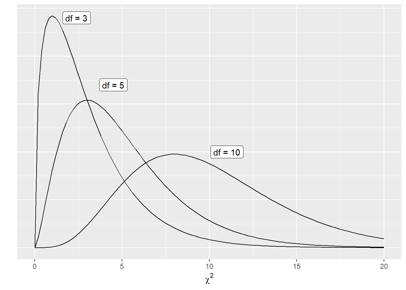
FIGURE 6.1: The chi-squared distribution with different degrees of freedom.
The calculated proportions within a two-way table represent the conditional distributions describing the relationships between both variables. In a chi-squared test, you describe the relationship by comparing the conditional distributions of the response variable (e.g., West Nile infection) for each level of the explanatory variable (e.g., the state where grouse were sampled). The hypotheses for the grouse example are then:
\(H_0\): West Nile infection and the state where grouse were sampled are independent.
\(H_A\): There is a relationship between West Nile infection and the state where grouse were sampled.
Before conducting the \(\chi^2\) test, we may be interested in calculating descriptive statistics that convey important information in the table. As an example, these can be the column or row percentages. A different number of grouse were sampled in each state, making it difficult to see trends across the three states. The prop.table() function turns counts into proportions:
prop.table(grouse)## West Nile Negative West Nile Positive
## Michigan 0.2565881 0.03883495
## Minnesota 0.3314840 0.04715673
## Wisconsin 0.2316227 0.09431345The addmargins() function will sum the proportions within each row and column. This makes it easier to see that nearly 82% of grouse test negative for West Nile and Minnesota had the largest number of grouse tested:
addmargins(prop.table(grouse))## West Nile Negative West Nile Positive Sum
## Michigan 0.2565881 0.03883495 0.2954230
## Minnesota 0.3314840 0.04715673 0.3786408
## Wisconsin 0.2316227 0.09431345 0.3259362
## Sum 0.8196949 0.18030513 1.0000000To work with the data more, first we can turn the grouse matrix into a tibble called grouse_df. Then, we will modify it to a long format to allow us to visualize it with ggplot():
grouse_df <- cbind(as_tibble(prop.table(grouse)),
                   State = c("Michigan","Minnesota","Wisconsin"))

grouse_df <- grouse_df %>%
  pivot_longer(!State, names_to = "Outcome", values_to = "Proportion")

grouse_df
## # A tibble: 6 x 3
## State Outcome Proportion
## <chr> <chr> <dbl>
## 1 Michigan West Nile Negative 0.257
## 2 Michigan West Nile Positive 0.0388
## 3 Minnesota West Nile Negative 0.331
## 4 Minnesota West Nile Positive 0.0472
## 5 Wisconsin West Nile Negative 0.232
## 6 Wisconsin West Nile Positive 0.0943The following graph plots a stacked bar graph showing the proportion of West Nile infections within each state. We observe that Wisconsin has a higher positive infection rate of West Nile compared to Michigan and Minnesota:
ggplot(grouse_df, aes(x = State, y = Proportion, fill = Outcome)) +
  geom_bar(stat = "identity", position = 'fill')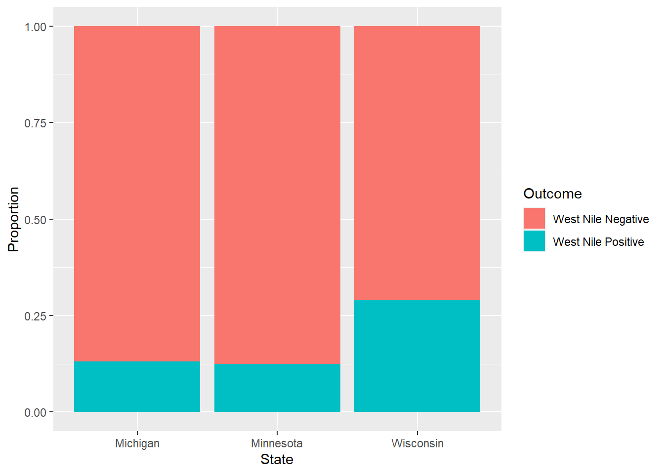
FIGURE 6.2: The distribution of West Nile infections in ruffed grouse across three states.
If we were to calculate the \(\chi^2\) statistic by hand, we would start by determining the expected cell counts. We will begin with grouse in Michigan that tested negative for West Nile. Recall that 213 grouse were from Michigan, 591 grouse tested negative for the virus, and 721 total grouse were sampled:
\[\text{expected}_\text{MI, Neg} = \frac{\text{row total} \cdot \text{column total}}{n}= \frac{213 \cdot 591}{721} = 174.6\]
So, we would expect 174.6 grouse in Michigan would test negative for West Nile. In the calculation of the \(\chi^2\) statistic we will compare this value to the observed number of grouse (185). We’ll then determine the expected number of grouse in Michigan that tested positive for West Nile:
\[\text{expected}_\text{MI, Pos} = \frac{213 \cdot 130}{721} = 38.4\]
Then we’ll calculate the expected cell counts for all other cells in the table:
\[\text{expected}_\text{MN, Neg} = \frac{273 \cdot 591}{721} = 223.8\]
\[\text{expected}_\text{MN, Pos} = \frac{273 \cdot 130}{721} = 49.2\]
\[\text{expected}_\text{WI, Neg} = \frac{235 \cdot 591}{721} = 192.6\]
\[\text{expected}_\text{WI, Pos} = \frac{235 \cdot 130}{721} = 42.4\]
Table 6.1 summarizes the observed and expected counts of the grouse data. The last column calculates the squared difference divided by the expected count and sums them to obtain the \(\chi^2\) statistic.
| State, Outcome | Observed | Expected | (Obs- Exp)^2 / Exp |
|---|---|---|---|
| MI, Neg | 185 | 174.6 | 0.62 |
| MI, Pos | 28 | 38.4 | 2.82 |
| MN, Neg | 239 | 223.8 | 1.03 |
| MN, Pos | 34 | 49.2 | 4.70 |
| WI, Neg | 167 | 192.6 | 3.40 |
| WI, Pos | 68 | 42.4 | 15.46 |
| SUM | 721 | 721.0 | 28.02 |
Note that the greatest value in the table of outcomes (15.46) is for grouse in Wisconsin that tested positive for the virus. This is due to the greater number of observed grouse with the virus (68) compared to the expected number (42.4). The greater proportion of infections in Wisconsin can also be seen in Figure 6.2. Minnesota saw a lower number of observed grouse with the virus (34) compared to the expected number (49.2). Together, these outcomes provide large values that go into the calculation of the \(\chi^2\) statistic.
The degrees of freedom for the grouse data are \((3-1)(2-1)=2\). With a \(\chi^2(2)\) distribution and a large value of the statistic (28.02), we will likely have evidence to support \(H_A\) and conclude that there is a relationship between West Nile infection and the state where grouse were sampled.
6.4 The chi-squared test in R
We were introduced to the chisq.test() function in Chapter 5 when we were dealing with data in a 2x2 table. The function is flexible to include any number of outcomes. For example, the grouse data are stored as a 3x2 table. If the data are stored in a matrix format, the chisq.test() function can be easily applied to run a chi-squared test at the \(\alpha = 0.05\) level:
chisq.test(grouse)##
## Pearson's Chi-squared test
##
## data: grouse
## X-squared = 28.094, df = 2, p-value = 7.935e-07Our manual calculation of the \(\chi^2\) statistic (28.02) produced a similar value to that provided by the function (28.094). Due to the small p-value (7.935e-07), we indeed have evidence to support \(H_A\) and conclude that there is a relationship between West Nile infection and the state where grouse were sampled.
6.4.1 Exercises
6.1 Determine the number of degrees of freedom for conducting a chi-squared test for the following case studies:
- A survey that asked participants their generation (Gen Z, Millennial, Gen X, or Boomer) and whether they have taken personal actions to address climate change in the last year (yes or no).
- A survey that asked participants their political party (conservative or liberal) and whether they believe that governments provide adequate funding to address climate change (yes or no).
- A survey that asked participants where they live (urban, rural, or suburban) and whether they believe governments should provide more, less, or the same amount of funding to address climate change.
6.2 Adedayo et al. (2010) investigated how rural women use forest resources in different regions in Nigeria. They surveyed women in three different ethnic groups according to different levels of income from forest resources, grouped in increments of 10%.
Run the code below to reproduce the data from Adedayo et al. (2010; their Table 2):
forest.resources <- matrix(c(2, 7, 22, 36, 10, 3,
                             5, 4, 20, 37, 8, 6,
                             0, 3, 28, 35, 10, 4),
                           ncol = 6, byrow = T)
colnames(forest.resources) <- c("<30%", "30--40%", "41--50%",
                                "51--60%", "61--70%", ">70%")
rownames(forest.resources) <- c("Yoruba", "Nupe", "Berom")- How many degrees of freedom are associated with a chi-squared test for these data?
- Run code in R that tests the null hypothesis that the proportion of respondents’ income from forest resources is independent from ethnic group at the \(\alpha=0.05\) level. State the results of the test in a sentence or two.
6.3. Run a similar chi-square test as above, but add the simulate.p.value = TRUE statement to the test. Research what this statement does by looking up the documentation for the chisq.test() function. How do the results of your test differ?
6.5 Summary
In the last chapter we learned about hypothesis tests for proportions. This was straightforward because we could analyze the data for two outcomes and two groups. Two-way tables extend this analysis by quantifying differences for any number of groups. Data that can be organized into two-way tables are widespread in natural resources and easy to visualize and interpret.
The chi-squared test and the statistic it provides measures how far the true counts are in a group/outcome and compares it to what we expect the number of counts to be. In doing this, hypotheses in chi-squared tests are set up to infer whether the groups are independent (the null hypothesis) or if there is a relationship between the groups (the alternative hypothesis). Base functions in R such as prop.table() and addmargins() allow you to explore and visualize two-way tables while the chisq.test() function performs chi-squared tests.