Chapter 5 Inference for counts and proportions
5.1 Introduction
One of the most common forms of quantitative data in natural resources are counts and proportions. This might include whether or not a species is present or absent in an area, whether a plant survived or died after an experimental treatment, or whether a rain event led to flood conditions or not.
In Chapter 3 we learned about the Bernoulli and binomial distributions, two discrete distributions that are common across natural resources. Counts of events and distributions can be modeled with the binomial distribution, so we will continue to use them in hypothesis tests with data collected as counts and proportions. What will make our jobs easier is to apply a normal approximation to make inferences about the proportion of successes in a population. When working with counts and proportions, it is critical to use the correct methods and analyses in R to make the appropriate inference on the population of interest.
5.2 The normal approximation for a binomial distribution
When the same chance process is repeated several times, we are often interested in whether a particular outcome happens on each repetition. In some cases, the number of repeated trials is fixed in advance and we are interested in the number of times a particular event (or a “success”) occurs. Recall from Chapter 3 that a binomial distribution is a series of Bernoulli trials n with probability of success p. Hence, the mean and variance of the binomial distribution is np and np(1-p), respectively.
Listed below are the four conditions of a binomial distribution. Moore et al. (2017) propose to think of BINS as a reminder of these conditions:
- Binary. All possible outcomes of each trial can be classified as “success” or “failure.”
- Independent. Trials must be independent; that is, knowing the result of one trial must not have any effect on the result of another.
- Number. The number of trials n of the chance process must be fixed in advance.
- Success. In each trial, the probability p of success must be the same.
The normal distribution allows us to make inference using several procedures and assumptions outlined in previous chapters. Fortunately, a normal approximation can be applied to a binomial distribution if n is relatively large. If \(np \geq 10\) and \(n(1-p) \geq 10\), we can apply the normal approximation to the binomial distribution.
As an example, consider that you are tasked with inspecting company facilities that store hazardous waste as a part of their operations. The probability of issuing a violation to the company for not following hazardous waste storage regulations is p = 0.24. We can confirm the data are binomial in their design: each facility is issued a violation or not (binary), inspections do not rely on the outcome of other inspections (independent), the number of inspections is fixed (as seen in the example below), and the probability of “success” is the same (e.g., the 24% chance a company is issued a violation).
Imagine you inspect 8, 20, and 80 facilities that result in the following distributions:
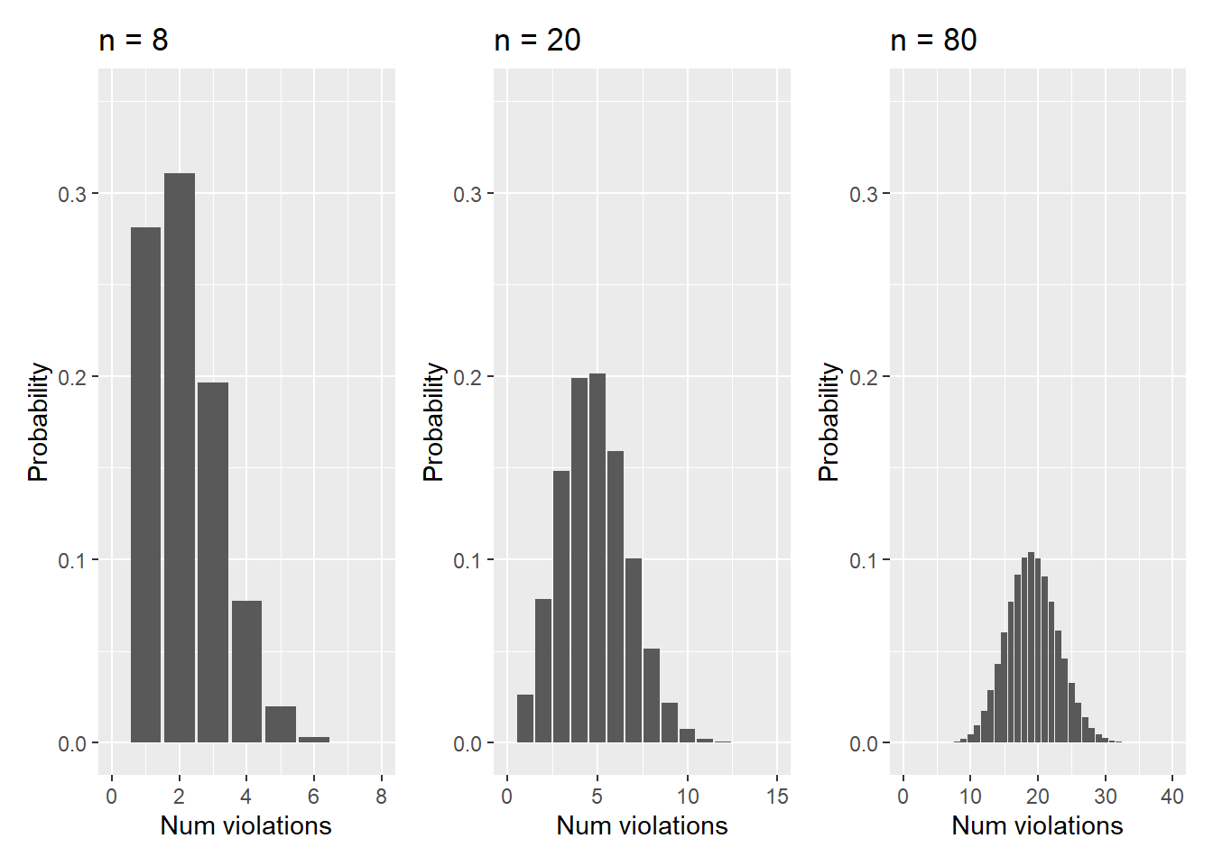
FIGURE 5.1: Hazardous waste violation probabilities with n = 8, 20, and 80.
Note that when n increases from 8 to 80, the distribution begins to approximate a normal distribution. We can determine the normal distribution approximation can be used in each of the scenarios:
- For n = 8, \(np = 8*0.24 = 1.9\) and \(n(1-p) = 8*(1-0.24) = 6.0\),
- For n = 20, \(np = 20*0.24 = 4.8\) and \(n(1-p) = 20*(1-0.24) = 15.2\), and
- For n = 80, \(np = 80*0.24 = 19.2\) and \(n(1-p) = 80*(1-0.24) = 60.8\).
Hence, only for n = 80 can we apply the normal approximation because \(np \geq 10\) and \(n(1-p) \geq 10\).
5.2.1 Exercises
5.1 Write a function in R that determines whether or not you can apply the normal distribution approximation for a given set of parameters n and p from a binomial distribution. Then, use that function to determine whether or not you can apply the approximation based on the following scenarios.
- You plant 10 tree seedlings with a known survival rate 85% after the first growing season.
- You plant 90 tree seedlings with a known survival rate 85% after the first growing season.
- You sample 20 ruffed grouse with a probability having West Nile virus of 0.13.
- There is a 40% chance of hearing a golden-winged warbler on a birding trip. You make 25 visits.
5.2 The code below uses ggplot() to produce a plot of the number of hazardous waste violations when \(n = 80\) and \(p = 0.24\). Change the arguments in the code to produce two plots showing the distribution of survival of 10 and 90 tree seedlings, each with a known survival rate of 85% after the first growing season. In particular, modify the scale_x_continuous() and scale_y_continuous() arguments to “zoom in” on the distribution.
x.80 <- 0:80
df.80 <- tibble(x = x.80, y = dbinom(x.80, 80, 0.24))

p.80 <- ggplot(df.80, aes(x = x.80, y = y)) +
  geom_bar(stat = "identity") +
  scale_x_continuous(limits = c(0, 40)) +
  scale_y_continuous(limits = c(0, 0.35)) +
  labs(title = "n = 80",
       x = "Number of violations",
       y = "Probability")
5.3 Sampling distribution and one-sample hypothesis test
Just like we looked at the sampling distribution of a mean value in Chapter 4, we can look at the sampling distribution of a proportion. Here, the sample statistic \(\hat{p}\) is used to estimate \(p\), the population proportion. The standard deviation of \(\hat{p}\) is
\[\sigma_{\hat{p}}=\sqrt{\frac{p(1-p)}{n}}\]
Since we’re interested in the population parameter \(p\), we can replace \(p\) with \(\hat{p}\) to find the standard error of the sample proportion:
\[\sigma_{\hat{p}}=\sqrt{\frac{\hat{p}(1-\hat{p})}{n}}\]
For sample proportions, we use the z-distribution for making inference about population parameters:
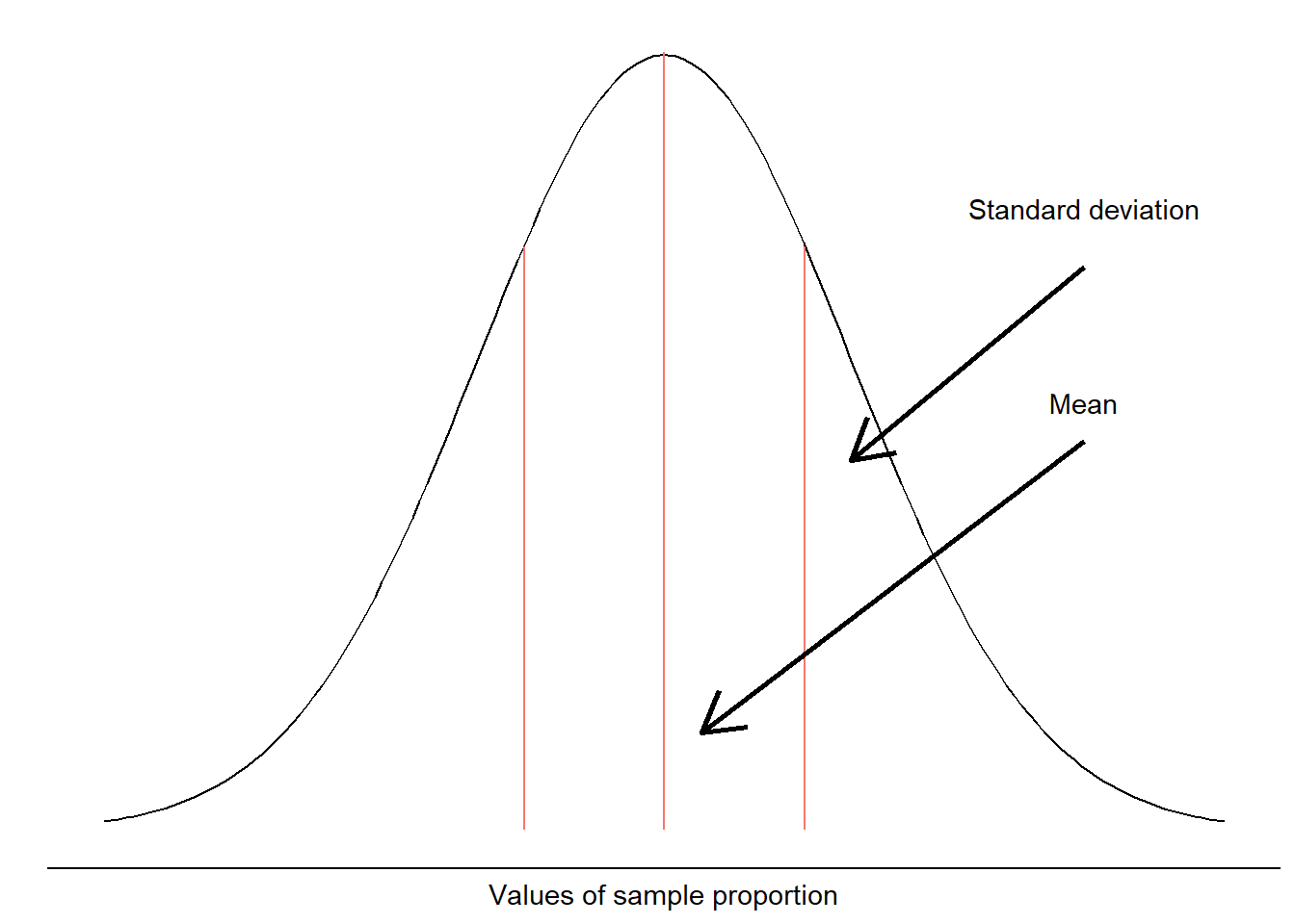
FIGURE 5.2: The sampling distribution of a sample proportion.
The null hypothesis for a one=sample proportion test can be written as \(H_0: p=p_0\), where \(p_0\) is a proportion we’re testing against. The following alternative hypotheses can be specified in a one-sample test for a proportion:
- \(H_A: p<p_0\) (left-tailed test)
- \(H_A: p>p_0\) (right-tailed test)
- \(H_A: p\neq p_0\) (two-tailed test)
Using the z-distribution, we calculate a statistic for this hypothesis test as:
\[z=\frac{\hat{p}-p}{\sqrt{\frac{p_0(1-p_0)}{n}}}\]
In R, two functions perform one-sample hypothesis tests for proportions. The prop.test() function applies the normal approximation to the binomial distribution and should be used when those conditions are met. The binom.test() is designed for smaller samples and should be used when the normal approximation conditions are not met.
For example, consider an organization that wants to make the claim that the majority of farmers (>50% of them) support limiting their use of nitrogen in their practices. While adding nitrogen in the form of fertilizer can improve the growth of crops, it can also run off into unintended water bodies. A polling company surveyed 30 farmers and their results indicated 18 of them supported limiting their use of nitrogen.

FIGURE 5.3: Application of nitrogen fertilization on a row crop. Image: University of Minnesota Extension.
We will conduct a hypothesis test with the null hypothesis \(H_0: p = 0.5\) and the alternative hypothesis \(H_A: p > 0.5\). The test will use a level of significance \(\alpha = 0.10\).
Our proportion of successes is \(p = 18/30 = 0.6\), so because \(np = 30*0.6 = 18\) and \(n(1-p) = 30*(1-0.6) = 12\), the normal distribution approximation is confirmed and the prop.test() function can be used. To carry out this one-sided hypothesis test, we enter x = 18 successes (number of farmers that agree with the limitations), n = 30 total farmers, a null proportion p = 0.50, and alternative = "greater" because we’re examining if the majority of farmers agree with the limitations:
prop.test(x = 18, n = 30, p = 0.50,
          alternative = "greater", conf.level = 0.90)
##
## 1-sample proportions test with continuity correction
##
## data: 18 out of 30, null probability 0.5
## X-squared = 0.83333, df = 1, p-value = 0.1807
## alternative hypothesis: true p is greater than 0.5
## 90 percent confidence interval:
## 0.4666054 1.0000000
## sample estimates:
## p
## 0.6Results indicate a p-value of 0.1807, indicating the survey has little evidence to support the statement that the majority of farmers support limits of nitrogen use. Thus, we accept the null hypothesis. The output also provides a chi-squared value of 0.83333. For comparison, we can also input the same statistics using the binom.test() function:
binom.test(x = 18, n = 30, p = 0.50,
           alternative = "greater", conf.level = 0.90)
##
## Exact binomial test
##
## data: 18 and 30
## number of successes = 18, number of trials = 30, p-value =
## 0.1808
## alternative hypothesis: true probability of success is greater than 0.5
## 90 percent confidence interval:
## 0.4665663 1.0000000
## sample estimates:
## probability of success
## 0.6Note the p-values and lower bound for the confidence interval are slightly different in both functions.
5.3.1 Exercises
5.3 Perform the following hypothesis tests for proportions at a level of significance \(\alpha=0.05\) using the prop.test() function and the given parameters. State your conclusions in a sentence or two.
- In a survey of 600 residents, 54% indicated they supported mining in their county. Perform a test that examines if your results can state that the majority of residents support mining.
- A tree nursery ensures that planting their seedlings will result in at least 90% survival after two years of growth. You question these claims after measuring 250 seedlings and find 215 of them survived after two years. Perform a test that examines if your results support the nursery’s claims.
- You sample 54 ruffed grouse for West Nile virus and find 5 of them to have the disease. Historical data indicate you expect 13% of grouse to test positive for the virus. You want to make the claim that you observed a positive infection rate less than the historical average.
5.4 The Random Geographic Coordinates web page (https://www.random.org/geographic-coordinates/) uses randomness to select a set of geographic coordinates at any location on Earth. Use the website to generate a random coordinate and record whether it falls on land or water. Repeat this so that you have 20 random locations and whether they are on land or water.
Determine the proportion of Earth covered with water from your collection of 20 random samples. Now, do an internet search to find the true proportion of Earth covered in water. Use prop.test() to run two two-tailed hypothesis tests for proportions, one at 90% and the other at a 50% confidence level. The null hypothesis is that your sampled proportion is equal to the true proportion of Earth covered in water. Does the true proportion of Earth covered in water fall within the calculated confidence interval provided in the R output?
5.4 Two-sample hypothesis tests for proportions
Remember that when we switched from using the z to the t-distribution, we began using the sample standard deviation s as opposed to the population standard deviation \(\sigma\). Similar to two-sample hypothesis tests for means, proportions use the properties of the population standard deviation \(\sigma\) as the basis for their inference.
Two-sample hypothesis tests for proportions examine \(p_1\) and \(p_2\), two population parameters representing different groups. The difference between the two proportions is the value that is examined in these hypothesis tests. When data are sampled randomly from two groups, we can approximate the difference \(p_1-p_2\) with \(\hat{p}_1-\hat{p}_2\), each of which may have different sample sizes \(n_1\) and \(n_2\).
The z-distribution can similarly be used for making inference about the difference in sample statistics \(\hat{p}_1-\hat{p}_2\). The sample standard deviation of can be estimated by:
\[\sigma_{\hat{p_1}-\hat{p_2}}=\sqrt{\frac{p_1(1-p_1)}{n_1} + \frac{p_2(1-p_2)}{n_2}}\]
We need a way to estimate a combined or “pooled” proportion p, so we can combine the data from the two samples by dividing the number of successes in both samples by the total number collected by both samples and call it \(\hat{p}\).
The null hypothesis for a two-sample test for proportions can be written as \(H_0: p_1=p_2\). The z-statistic for this hypothesis test is:
\[z=\frac{\hat{p}_1-\hat{p}_2}{\sqrt{{\hat{p}(1-\hat{p})(\frac{1}{n_1}+\frac{1}{n_2})}}}\]
The following alternative hypotheses can be specified in two-sample tests for proportions:
- \(H_A: p_1-p_2<0\) (left-tailed test)
- \(H_A: p_1-p_2>0\) (right-tailed test)
- \(H_A: p_1-p_2\neq 0\) (two-tailed test)
The prop.test() function can also perform hypothesis tests that compare two sample proportions.
For example, consider an organization that wants to compare farmer support in limiting nitrogen use in two counties. In one county, a polling company surveyed 40 farmers and 19 of them supported limiting their use of nitrogen. In a different county, a polling company surveyed 36 farmers and 24 of them supported limited nitrogen use. We can specify these data as vectors:
farmer.support <- c(19, 24)
farmer.total <- c(40, 36)
So, our proportion of farmers that support limiting their nitrogen use is \(p_1 = 19/40 = 0.48\) and \(p_2 = 24/36 = 0.66\) in the first and second counties, respectively. We will conduct a hypothesis test with the null hypothesis \(H_0: p_1=p_2\) and the alternative hypothesis \(H_A: p_1-p_2\neq p_0\). The test will use a level of significance \(\alpha = 0.10\).
To carry out this two-sided hypothesis test, we enter both of the vectors that contain the data as the first two arguments:
prop.test(farmer.support, farmer.total,
          alternative = "two.sided", conf.level = 0.90)
##
## 2-sample test for equality of proportions with continuity
## correction
##
## data: farmer.support out of farmer.total
## X-squared = 2.1068, df = 1, p-value = 0.1466
## alternative hypothesis: two.sided
## 90 percent confidence interval:
## -0.40127198 0.01793865
## sample estimates:
## prop 1 prop 2
## 0.4750000 0.6666667Results indicate a p-value of 0.1466, indicating no difference between counties in farmer support for limiting nitrogen use. So, we accept the null hypothesis. Note that the 90% confidence interval provides upper and lower bounds around the mean difference between both proportions (0.1917).
When two samples contain either a success or failure, we can represent this in the form of a 2x2 table. The matrix() function allows us to view the data in a compact format. The column and row name labels can be renamed with colnames() and rownames(), respectively:
farmer.nitrogen <- matrix(c(19, 24, 21, 12), ncol = 2, byrow = T)
colnames(farmer.nitrogen) <- c("Support", "DoNotSupport")
rownames(farmer.nitrogen) <- c("County1", "County2")
farmer.nitrogen
## Support DoNotSupport
## County1 19 24
## County2 21 12For data in a 2x2 table like this, the chisq.test() function will provide the same results that prop.test() does. Note the minimal output provided using chisq.test() compared to the prop.test() function (e.g., no confidence interval or means of sample estimates):
chisq.test(farmer.nitrogen)##
## Pearson's Chi-squared test with Yates' continuity correction
##
## data: farmer.nitrogen
## X-squared = 2.1068, df = 1, p-value = 0.1466For small samples and low numbers of successes (typically fewer than five), the fisher.test() function is appropriate for comparing two sample proportions. This function also requires the data to be in a matrix format:
fisher.test(farmer.nitrogen,
            alternative = "two.sided", conf.level = 0.90)
##
## Fisher's Exact Test for Count Data
##
## data: farmer.nitrogen
## p-value = 0.1092
## alternative hypothesis: true odds ratio is not equal to 1
## 90 percent confidence interval:
## 0.187029 1.091269
## sample estimates:
## odds ratio
## 0.4572285Note the difference in the p-value for both tests (0.1466 and 0.1092) and the way in which the confidence interval differs. For the fisher.test() function, a confidence interval for the odds ratio is provided that compares the likelihood of \(p_1\) with \(p_2\). The 90% confidence interval for the odds ratio contains 1, indicating the proportions between farmer support of nitrogen use in each county is similar.
5.4.1 Exercises
5.5 Perform the following two-sample hypothesis tests for proportions at a level of significance \(\alpha=0.05\) using the prop.test() or chisq.test() functions and the given parameters. State your conclusions in a sentence or two.
- In a survey of 500 residents in each of two counties, 280 and 220 residents in each county indicated they supported mining. Perform a test that examines whether or not the proportion of support for mining differs in these counties.
- After planting 250 oak tree seedlings you find 215 of them survived after two years. After planting 175 maple tree seedlings you find 165 of them survived after two years. Perform a test that examines whether or not the proportion of surviving oak trees is less than the proportion of surviving maple trees.
- You sample 64 ruffed grouse for West Nile virus in Michigan and find 8 of them to have the disease. In a similar study in Wisconsin, 45 grouse were tested and 7 had the disease. Perform a test that examines whether or not the proportion of West Nile infections differs in these two states.
5.6 The air quality data set is a built-in data set in R that provides daily air quality measurements collected in New York City from May to September 1973.
Run the code below to read in the air quality data set. We’ll name the data set air using the tibble() function:
library(tidyverse)
air <- tibble(airquality)
Two variables in air that we will use are:
- Mean ozone in parts per billion from 1300 to 1500 hours at Roosevelt Island (
Ozone) - Numeric month from May through September (
Month)
Write R code to find the number of days when the ozone level was unhealthy for sensitive groups or greater, defined as an ozone measurement greater than or equal to 101. Then, perform a two-sample test of proportions that determines if the proportion of unhealthy air quality days was different between the spring (months of May and June) and summer (months of July, August, and September). Perform the tests at a level of significance \(\alpha=0.05\). NOTE: Do not include days with an NA for ozone measurement.
5.5 Summary
The general approach to hypothesis tests using proportions is similar to how we handled continuous data. The primary difference in the test for proportions is the use of the z rather than the t-statistic. Applying the normal approximation for a binomial distribution will allow us to make inference with data stored as counts and proportions. The prop.test() function allows us to perform many one- and two-sample hypothesis tests for proportions in R.
We’ll return to these concepts in Chapter 6 when we discuss chi-squared tests more in depth. There, you might imagine that we have more rows and columns, for example, if we asked farmers from three counties their opinion about nitrogen use and they could respond by stating that they support, do not support, or have no opinion on the topic (resulting in a 3x3 table). In the future, we will calculate the appropriate sample size that allows us to estimate a population proportion within a given margin of error, a calculation that has long been used in political and opinion polling.