Chapter 4 Hypothesis tests for means and variances
4.1 Introduction
This chapter will introduce the concepts of hypothesis tests. At their simplest, hypothesis tests are claims that we make about phenomena. Hypothesis tests are tools that allow us to make statements about whether or not the means or variances of data are equal to a unique value or whether or not two groups of data are different.
Now that we have a foundation of probability, hypothesis tests will make up a large component of how we use statistical tests to make inference about populations:
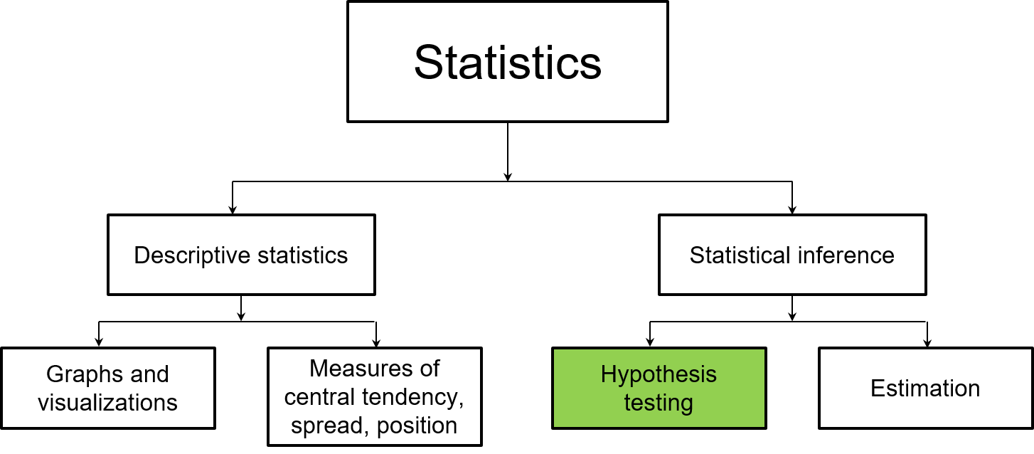
FIGURE 4.1: The next chapters focus on hypothesis tests, a component of statistical inference.
Recall that we use different notation to denote what we mean by the sample and the population. This is essential in hypothesis testing because we collect data from samples to inform differences across populations:
- For counts, the population parameter is represented by \(N\) and the sample statistic by \(n\).
- For the mean, the population parameter is represented by \(\mu\) and the sample statistic by \(\mu_{\bar{y}}\) or \(\bar{y}\).
- For the variance, the population parameter is represented by \(\sigma^2\) and the sample statistic by \(s^2\).
- For the standard deviation, the population parameter is represented by \(\sigma\) and the sample statistic by \(s\).
This chapter will provide an introduction to the theory and concepts behind hypothesis testing and will introduce two new distributions to compare the mean and variance of a variable of interest.
4.2 Statistical significance and hypothesis tests
A test of statistical significance is a formal procedure for comparing observed data with a claim whose truth we want to assess. For example, consider a sample that determined the average size of a pack of wolves to be 4.8 wolves. A wildlife biologist is skeptical of this finding, claiming that she believes the average wolf pack size is seven wolves. Is the mean value of 4.8 significantly different from 7 wolves? Consider if wolf pack sizes in a different area were sampled with a mean size of 3.5 wolves. Are 4.8 and 3.5 wolves significantly different from each other?
A test of statistical significance evaluates a statement about a parameter such as the population mean \(µ\) or variance \(\sigma^2\). The results of a significance test are expressed in terms of a probability termed the p-value. A p-value is the probability under a specified statistical model that a statistical summary of the data would be equal to or more extreme than its observed value. P-values do not measure the probability that a hypothesis is true nor should scientific conclusions or decisions be made if the p-values fall below or above some threshold value (Wasserstein and Lazar 2016). We will use statistical tests and the p-values that result from them as another metric when we perform hypothesis tests.
Any significance test begins by stating the claims we want to compare. These claims are termed the null and alternative hypotheses. The null hypothesis, denoted \(H_0\), is the hypothesis being tested. The null hypothesis is assumed to be true, but your data may provide evidence against it. The alternative hypothesis, denoted \(H_A\) is the hypothesis that may be supported based on your data. Every hypothesis test results in one of two outcomes:
- The null hypothesis is rejected (i.e., the data support the alternative)
- The null hypothesis is accepted, or we fail to reject the null hypothesis (i.e., the data support the null)
When we draw a conclusion from a test of significance (assuming our null hypothesis is true), we hope it will be correct. However, due to chance variation, our conclusions may sometimes be incorrect. Type I error and Type II error are two ways that measure the error associated with hypothesis tests.
- Type I error occurs when we reject the null hypothesis when it is in fact true. Type I error reflects the level of significance of a hypothesis test, denoted by \(\alpha\).
- Type II error occurs when we fail to reject the null hypothesis when it is in fact false, denoted by \(\beta\).
The complements of both Type I and Type II errors represent the correct decisions of a hypothesis test. The probability of correctly rejecting the null hypothesis is when it is indeed false is \(1-\beta\), also known as the statistical power of a hypothesis test.
4.2.1 Setting up hypothesis tests
Hypothesis tests can be one- or two-tailed. This choice depends on how the null hypotheses are set up. For example, consider a one-sample t-test for a mean, which will be described more in depth later in this chapter. This test compares the difference between a mean value \(\mu\) and a hypothesized value in the population. This hypothesized mean is often a unique or interesting value that we wish to compare to, denoted \(\mu_0\).
Our null hypothesis can be written as \(H_0: \mu=\mu_0\). The following alternative hypotheses can be specified:
- \(H_A: \mu<\mu_0\). This is a left-tailed test.
- \(H_A: \mu>\mu_0\). This is a right-tailed test.
- \(H_A: \mu\neq\mu_0\). This is a two-tailed test.
If a p-value falls within the critical region for the left- and right-tailed tests (to the left or right area of the distribution, respectively), the null hypothesis is rejected. For the same level of significance, say \(\alpha = 0.05\), we will “split the difference” for a two-tailed test. If a p-value falls inside the left or right tails in a two-tailed test, the null hypothesis is rejected. Notice the smaller critical regions on both sides of the distribution for a two-tailed test.
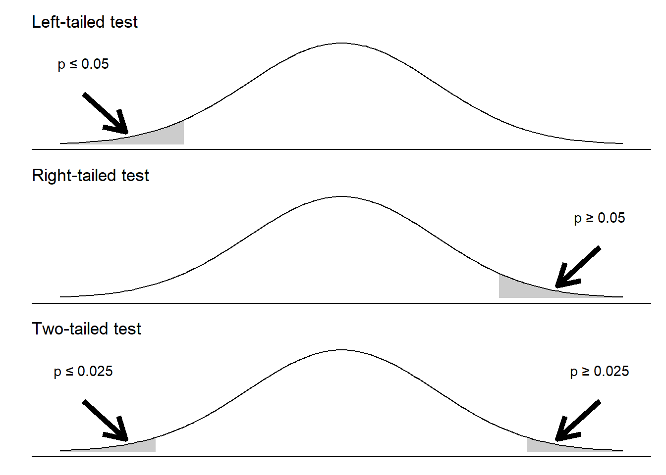
FIGURE 4.2: Conclusions of different alternative hypotheses with a level of significance of 0.05.
4.2.2 The Student’s t-distribution
The Student’s t-distribution is a continuous probability distribution that assumes a normally distributed population and an unknown standard deviation. The distribution and associated tests were developed by William Sealy Gosset in the early 1900s, a story with a rich history that is told in the popular book The Lady Tasting Tea (Salsburg 2001).
The t-distribution is similar in shape to a normal distribution but is less peaked with wider tails. The t-distribution works well with small samples because the sample standard deviation \(s\) can be used. (We do not know the population standard deviation \(\sigma\) which differentiates it from the z-distribution.)
The shape of the t-distribution depends on its degrees of freedom. The degrees of freedom (df) are the minimum number of independent values needed to specify a distribution. Degrees of freedom vary depending on the number of samples. When we make inference about a population mean \(\mu\) using a t-distribution, the appropriate degrees of freedom are found by subtracting 1 from the sample size \(n\). Hence \(df = n – 1\). As the degrees of freedom increase, the t density curve more closely resembles the standard normal distribution.
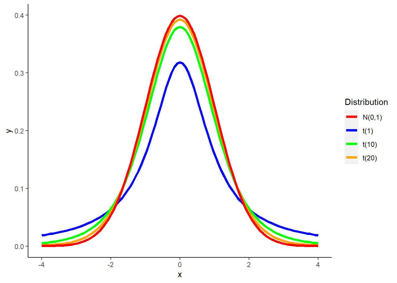
FIGURE 4.3: The Student’s t-distribution with different degrees of freedom compared to the standard normal N(0,1) distribution.
4.2.3 Confidence intervals
Related to the two-tailed hypothesis test and the t-distribution is the confidence interval. A confidence interval has a lower and upper bound that contains the true value of a parameter. A 95% confidence level is most commonly used across disciplines, corresponding to a level of significance of \(\alpha = 0.05\).
If we sample from a population with an approximate normal distribution, a confidence interval can be calculated as:
\[\bar{y}\pm{t_{n-1, \alpha/2}}\frac{s}{\sqrt{n}}\]
where \(\bar{y}\) is the mean of the sample, \(t_{n-1, \alpha/2}\) is the value t from the t-distribution, \(s\) is the standard deviation, and \(n\) is the number of observations.
In R, the qt() function allows us to calculate the correct value of t to use. This function provides the quantiles of the t-distribution if we specify the quantile we’re interested in and the number of degrees of freedom. As an example, we could use the following code to find the t-statistic for the 95th quantile of the t-distribution with 9 degrees of freedom.
qt(0.95, df = 9)## [1] 1.833113Consider we want to calculate a 95% confidence interval on the number of chirps that a striped ground cricket makes, a data set we saw in Chapter 2 (chirps). The data contain the number of chirps per second (cps) and the air temperature measured in degrees Fahrenheit (temp_F):
library(stats4nr)

head(chirps)
## # A tibble: 6 x 2
## cps temp_F
## <dbl> <dbl>
## 1 20 93.3
## 2 16 71.6
## 3 19.8 93.3
## 4 18.4 84.3
## 5 17.1 80.6
## 6 15.5 75.2To find a 95% confidence interval for the number of chirps we will calculate the mean, standard deviation, and number of observations. Notice how we specify the values in the qt() function to provide the appropriate values to obtain the confidence levels:
mean_cps <- mean(chirps$cps)
sd_cps<- sd(chirps$cps)
n_cps<- length(chirps$cps)

low_bound <- mean_cps + (qt(0.025,
                            df = n_cps - 1) *
                           (sd_cps / sqrt(n_cps)))
high_bound <- mean_cps + (qt(0.975,
                             df = n_cps - 1) *
                            (sd_cps / sqrt(n_cps)))
low_bound; high_bound
## [1] 15.71077## [1] 17.59589So, we can state that the 95% confidence interval for the number of chirps is [15.71, 17.60]. In application, this means that if we collected another 100 samples of the number of chirps from striped ground crickets, 95 of the means would fall within this confidence interval.
Note that we can change the quantile to calculate a narrower confidence interval. For example, we can use the chirps data to compute a 90% confidence interval by changing the quantile in the qt() function:
low_bound_90 <- mean_cps + (qt(0.05,
                               df = n_cps - 1) * (sd_cps / sqrt(n_cps)))
high_bound_90 <- mean_cps + (qt(0.95,
                               df = n_cps - 1) * (sd_cps / sqrt(n_cps)))
low_bound_90; high_bound_90
## [1] 15.8793## [1] 17.42737So, we can state that the 90% confidence interval for the number of chirps is [15.87, 17.43].
DATA ANALYSIS TIP Andrew Gelman, professor of statistics and political science at Columbia University, has reported interesting results about confidence intervals. He has observed that when people are asked to provide levels of uncertainty, their 50% intervals are typically correct 30% of the time. When people provide 90% levels of uncertainty, their intervals are typically correct 50% of the time. This is, in part, why some prefer to use narrower intervals, such as at the 50% level (Gelman 2016).
4.2.4 Exercises
4.1 Use R to calculate the t-statistic at the following quantiles with various degrees of freedom.
- The 10th quantile with 8 degrees of freedom.
- The 10th quantile with 16 degrees of freedom.
- The 75th quantile with 10 degrees of freedom.
- The 90th quantile with 22 degrees of freedom.
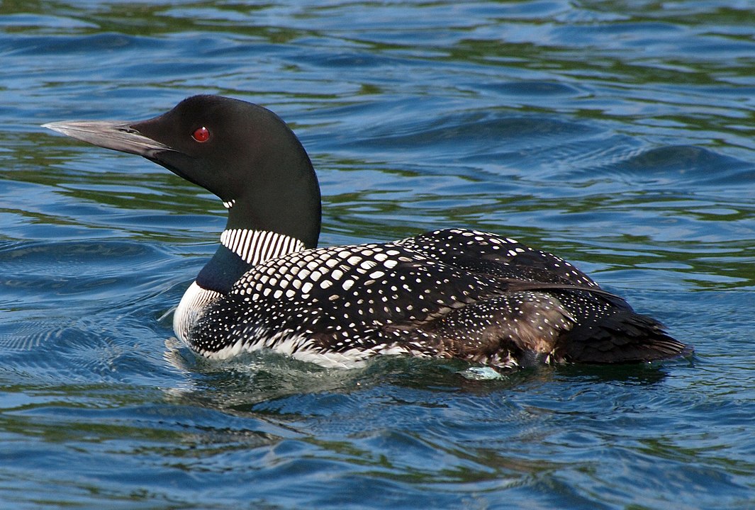
FIGURE 4.4: A common loon. Image: John Picken.
4.2 Mercury is a highly mobile contaminant that can cycle through air, land, and water. The mercury content of 60 eggs were measured from nests of common loons (Gavia immer), a diving bird, in New Hampshire, USA (Loon Preservation Committee 1999). They calculated a mean of \(\bar{y}=0.540\) parts per million (ppm) and a standard deviation \(s=0.399\) ppm. Use these summary statistics to answer the following questions.
- Use R code to calculate a 95% confidence interval around the mean mercury content of the loon eggs.
- Calculate an 80% confidence interval around the mean mercury content of the loon eggs.
- Wildlife biologists know that elevated mercury content of loon eggs occurs when mercury content is greater than 0.5 ppm. Reproductive impairment of loon eggs occurs when mercury content is greater than 1.0 ppm. Where do these values fall within both of the confidence intervals you calculated?
4.3 Fisheries biologists measured the weight of yellow perch (Perca flavescens), a species of fish. Data were from a sample from a population of yellow perch in a lake. They calculated a mean perch weight of 260 grams and a variance of 10,200 after measuring a sample of 18 perch. Use R code to calculate a 90% confidence interval around the mean perch weight.
4.3 Hypothesis tests for means
4.3.1 One-sample t-test for a mean
A t-statistic can be calculated for a hypothesis test about a population mean \(\mu\) with unknown population standard deviation \(\sigma\). The value for the t-statistic represents how many standard errors a sample mean \(\bar{y}\) is from a hypothesized mean. In a one-sample t-test for a mean, the t-statistic is calculated by comparing the sample mean \(\bar{y}\) to a hypothesized mean \(\mu_0\) (in the numerator) and dividing it by the standard error (in the denominator):
\[t=\frac{\bar{y}-\mu_0}{s/\sqrt{n}}\]
In R, the t.test() function performs a number of hypothesis tests related to the t-distribution. For example, assume an entomologist makes a claim that a striped ground cricket makes 18 chirps per second. We can perform a two-sided one-sample t-test at a level of significance of \(\alpha = 0.05\) that compares our sample with this value under the following hypotheses:
- The null hypothesis (\(H_0\)) states that the true mean of the number of chirps a striped ground cricket makes is equal to 18.
- The alternative hypothesis (\(H_A\)) states that the true mean of the number of chirps a striped ground cricket makes is not equal to 18.
This can be determined by specifying the sample data and the value being tested against in the mu = statement:
t.test(chirps$cps, mu = 18)##
## One Sample t-test
##
## data: chirps$cps
## t = -3.0643, df = 14, p-value = 0.008407
## alternative hypothesis: true mean is not equal to 18
## 95 percent confidence interval:
## 15.71077 17.59589
## sample estimates:
## mean of x
## 16.65333The calculated t-statistic is -3.0643 with 14 degrees of freedom. The p-value of 0.008407 is less than our level of significance of \(\alpha = 0.05\). Hence, we can conclude that we have evidence to reject the null hypothesis and conclude that the true mean of the number of chirps a striped ground cricket makes is not equal to 18.
Also provided in the R output is the mean number of chirps (16.6533) and the 95% confidence interval (15.71077, 17.59589). Our sample mean was less than our hypothesized mean in this one-sample t-test.
The conf.level statement allows you to change the confidence level, corresponding to the complement of the level of significance. For example, we could run the same hypothesis test at a level of significance of 0.10:
t.test(chirps$cps, mu = 18, conf.level = 0.90)##
## One Sample t-test
##
## data: chirps$cps
## t = -3.0643, df = 14, p-value = 0.008407
## alternative hypothesis: true mean is not equal to 18
## 90 percent confidence interval:
## 15.87930 17.42737
## sample estimates:
## mean of x
## 16.65333Notice that while the conclusion of the hypothesis test does not change, the confidence interval is narrower at a more liberal level of significance.
By default the t.test() function will run a two-tailed hypothesis test. To specify a one-sided test, you can use the alternative statement:
- Use
alternative = "less"for a left-tailed test when \(H_A: \mu<\mu_0\). - Use
alternative = "greater"for a right-tailed test when \(H_A: \mu>\mu_0\).
t.test(chirps$cps, mu = 18, alternative = "greater")##
## One Sample t-test
##
## data: chirps$cps
## t = -3.0643, df = 14, p-value = 0.9958
## alternative hypothesis: true mean is greater than 18
## 95 percent confidence interval:
## 15.8793 Inf
## sample estimates:
## mean of x
## 16.65333t.test(chirps$cps, mu = 18, alternative = "less")##
## One Sample t-test
##
## data: chirps$cps
## t = -3.0643, df = 14, p-value = 0.004204
## alternative hypothesis: true mean is less than 18
## 95 percent confidence interval:
## -Inf 17.42737
## sample estimates:
## mean of x
## 16.65333Notice the differences in outcomes in the two hypothesis tests. The sample mean \(\bar{y} = 16.65\) is less that the hypothesized mean \(\mu_0 = 18\), so we have evidence to conclude that the true population mean is not greater than 18, but is less than 18. The other important output to note when using the alternative statement is the Inf and -Inf values for the confidence intervals. This is the result of the one-sided test that was specified with no lower and upper bounds.
NONPARAMETRIC STATISTICS: Most of what we discuss in this chapter falls under the family of parametric statistics, which assume that the data sampled can be modeled with a probability distribution. Another family, termed nonparametric statistics or distribution-free methods, make no prior assumption that data reflect a probability distribution. The nonparametric equivalent of the t-test is termed the Wilcoxon test. In this test, the distribution is considered symmetric around the hypothesized mean (e.g., 18 with the chirps data). The differences between the data and the hypothesized mean are calculated and ranked to determine the test statistic. With the chirps data, try running
wilcox.test(chirps$cps, mu = 18)and compare the output with thet.test()function. For more on nonparametric statistics, Kloke and McKean (2014) is an excellent reference.
4.3.2 Two-sample t-test for a mean
A two sample t-test is used if we want to compare the means of a quantitative variable for two populations. In this case, our parameters of interest are the population means \(\mu_1\) and \(\mu_2\). Similar to a one-sample test, random samples can be obtained to compare the sample means.
With two-sample hypothesis tests, we’ll need to understand the properties of the population standard deviation \(\sigma\). With two populations, their standard deviations \(\sigma_1\) and \(\sigma_2\) may be equal or unequal to one another. That result will influence how the t-statistic is calculated.
The primary assumptions before performing a two-sample t-test for a mean are as follows:
- The two samples are independent of one another. That is, one observation is not influenced by another.
- The data follow a normal distribution.
There are two versions of t-tests that assess the difference between two means: the pooled and Welch t-test.
4.3.2.1 Pooled t-test
Assuming the two population standard deviations are equal, a pooled t-test calculates a two-sample t-statistic as:
\[t=\frac{\bar{y}_1-\bar{y}_2}{\sqrt{\frac{s^2}n_1+\frac{s^2}n_2}}\]
where \(\bar{y}_1\), \(\bar{y}_2\), \(n_1\), and \(n_2\) represent the means and number of samples for the first and second groups. The variance \(s^2\) is an estimate of the sample variance that is obtained by “pooling” the sample variances from both samples. The degrees of freedom for the test are calculated as \(n_1+n_2-2\).
To conduct a two-sample pooled t-test, let’s add a simulated sample of the number of chirps per second to the chirps data set. We do this by using add_column(), a tidyverse function:
chirps <- chirps %>%
  add_column(cps_2 = c(20.5, 16.3, 20.9, 18.6, 17.5, 15.7,
                       14.9, 17.5, 15.9, 16.5, 15.3, 17.7,
                       16.2, 17.6, 14.6))
After rearranging the data to a long format with pivot_longer(), notice the slightly larger values in cps_2 compared to cps:
chirps2 <- chirps %>%
  pivot_longer(!temp_F, names_to = "dataset", values_to = "cps")

ggplot(chirps2, aes(dataset, cps)) +
  geom_boxplot() +
  labs(x = "Data set", y = "Chirps per second")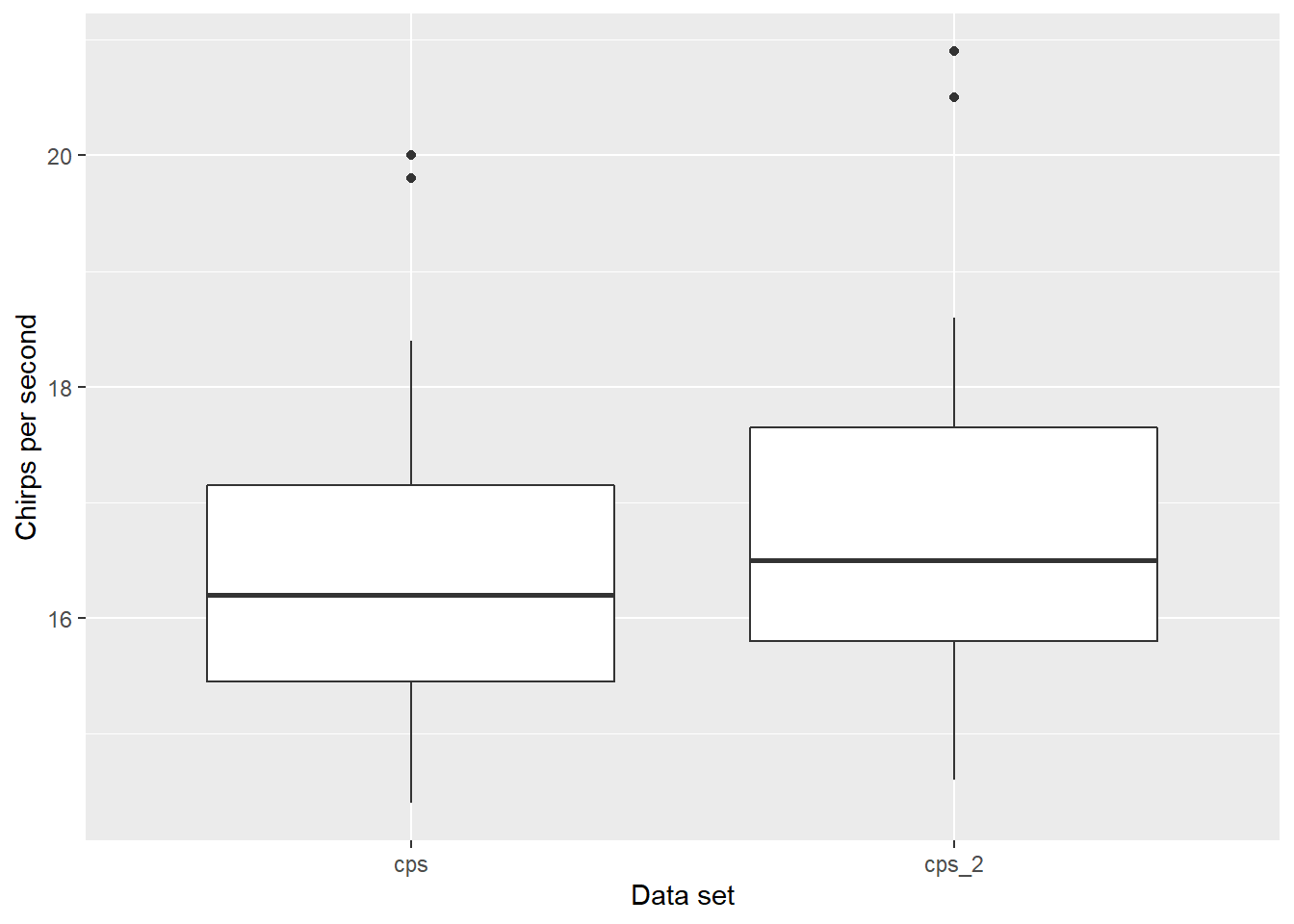
The t.test() function can also be specified for two-sample t-tests. We can specify a two-sided two-sample t-test at a level of significance of \(\alpha = 0.05\) that determines whether or not the two populations of ground cricket chirps are equal with the following hypotheses:
- The null hypothesis (\(H_0\)) states that the true mean of the number of chirps a striped ground cricket makes in
cpsis equal tocps_2. - The alternative hypothesis (\(H_A\)) states that true mean of the number of chirps a striped ground cricket makes in
cpsis not equal tocps_2.
The following is an example of the pooled t-test assuming variances are equal at a level of significance of \(\alpha = 0.05\):
t.test(chirps$cps, chirps$cps_2, conf.level = 0.95, var.equal = TRUE)##
## Two Sample t-test
##
## data: chirps$cps and chirps$cps_2
## t = -0.6034, df = 28, p-value = 0.5511
## alternative hypothesis: true difference in means is not equal to 0
## 95 percent confidence interval:
## -1.728617 0.941950
## sample estimates:
## mean of x mean of y
## 16.65333 17.04667Note that the calculated t-statistic is -0.6034 with 28 degrees of freedom. The p-value of 0.5511 is greater than our level of significance of \(\alpha = 0.05\). Hence, we have evidence to accept the null hypothesis and conclude that the true mean of the number of chirps a striped ground cricket makes in cps is equal to cps_2.
4.3.2.2 Welch t-test
Assuming the two population standard deviations are not equal, a Welch t-test calculates a two-sample t-statistic as:
\[t=\frac{\bar{y}_1-\bar{y}_2}{\sqrt{\frac{s_1^2}n_1+\frac{s_2^2}n_2}}\]
where \(\bar{y}_1\), \(\bar{y}_2\), \(s_1^2\), \(s_2^2\), \(n_1\), and \(n_2\) represent the means, variances, and number of samples for the first and second groups. Notice how the variances from each sample are used directly in this calculation. The degrees of freedom for the Welch test is a more complex calculation using the variance and number of observations from each sample.
We can assume the same hypothesis test comparing means of cps and cps_2. The following is an example of the Welch t-test assuming variances are not equal at a level of significance of \(\alpha = 0.05\):
t.test(chirps$cps, chirps$cps_2, conf.level = 0.95, var.equal = FALSE)##
## Welch Two Sample t-test
##
## data: chirps$cps and chirps$cps_2
## t = -0.6034, df = 27.77, p-value = 0.5511
## alternative hypothesis: true difference in means is not equal to 0
## 95 percent confidence interval:
## -1.7291150 0.9424483
## sample estimates:
## mean of x mean of y
## 16.65333 17.04667Note that the t-statistic and p-values are the same for both tests. However, the degrees of freedom are slightly lower in the Welch t-test (27.77) compared to the pooled t-test (28). For this relatively small data set, this results in slight differences in the lower and upper bounds of the confidence intervals. Before deciding whether to use the pooled or Welch test, consult the procedures outlined in the Hypothesis tests for variances section later in this chapter.
4.3.3 Paired t-test
Two samples are often dependent on one another, that is, one observation is influenced by the other. A paired t-test evaluates the difference between the responses of two paired measurements.
When paired data result from measuring the same quantitative variable twice, the paired t-test analyzes the differences in each pair. For example, consider a survey designed to examine hunter attitudes to new hunting policies. Ten hunters take a survey on their knowledge of new policies, then listen to a presentation that describes the new policies in detail. After the presentation the hunters take a similar survey on their knowledge. In this example a paired t-test is appropriate because the two samples are dependent, that is, the same hunters are being surveyed.
The paired t-test is similar in design to a one-sample t-test. Instead, the differences of the two means are evaluated. We will first find the mean difference (\(\bar{d}\)) between the responses within each pair \(\bar{y}_1\) and \(\bar{y}_2\). Then we will calculate the test statistic to evaluate these differences:
\[t=\frac{\bar{d}-\mu_d}{s_d/\sqrt{n}}\] where \(\mu_d\) is a value to be tested against (typically 0), \(s_d\) is the standard deviation of the difference, and \(n\) is the number of pairs.
For example, assume a group of eight hunters were first asked how many days they would spend afield during a hunting season. Then, the same hunters listened to a presentation by a wildlife biologist describing new hunting regulations that would adjust the number of opening and closing dates of the hunting season by geographic regions, ultimately leading to a longer hunting season. The hunters again estimated how many days they would spend afield after the new regulations took place. Here are the data represented in the days variables:
hunt <- tribble(
  ~hunterID, ~time, ~days,
  1, " Pre", 5,
  2, " Pre", 7,
  3, " Pre", 3,
  4, " Pre", 9,
  5, " Pre", 4,
  6, " Pre", 1,
  7, " Pre", 6,
  8, " Pre", 2,
  1, "Post", 8,
  2, "Post", 7,
  3, "Post", 4,
  4, "Post", 11,
  5, "Post", 9,
  6, "Post", 3,
  7, "Post", 10,
  8, "Post", 5
)

ggplot(hunt, aes(time, days)) +
  geom_boxplot() +
    geom_point() +
  labs(x = "Time period",
       y = "Estimated days to hunt")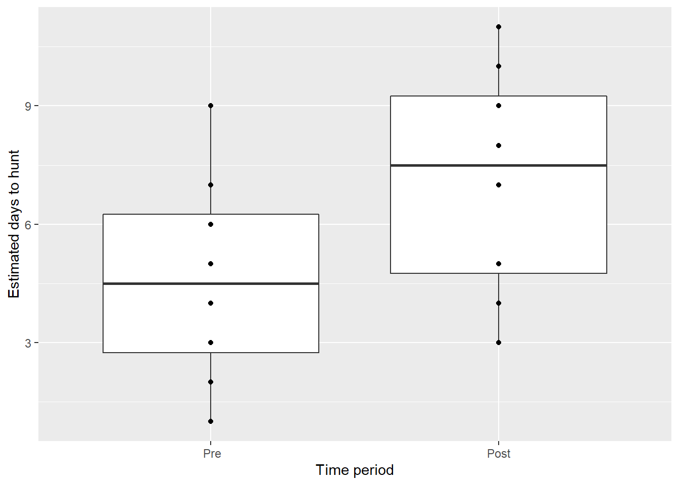
Our null hypothesis can be written as \(H_0: \mu_d = 0\) and alternative hypothesis \(H_A: \mu_d\neq0\). After filtering the pre and post measurements, we can specify the paired = TRUE statement to the t.test() function to perform a paired t-test:
pre <- hunt %>%
  filter(time == " Pre")

post <- hunt %>%
  filter(time == "Post")

t.test(pre$days, post$days, paired = TRUE)
##
## Paired t-test
##
## data: pre$days and post$days
## t = -4.4096, df = 7, p-value = 0.00312
## alternative hypothesis: true difference in means is not equal to 0
## 95 percent confidence interval:
## -3.840616 -1.159384
## sample estimates:
## mean of the differences
## -2.5The t-statistic is -4.41 and p-value is 0.00312 with 7 degrees of freedom. On average, hunters estimated they would spend 2.5 more days in the field after listening to the presentation. Hence, we have evidence to reject the null hypothesis.
4.3.4 Exercises
4.4 For the following questions, use the elm data set.
- Use R to calculate the mean, standard deviation, number of observations, and standard error of the mean for the mean of tree height (
HT). - Calculate a 95% confidence interval for the population mean of tree height (
HT) from the elm data set. Interpret the meaning of the confidence interval and what it is telling you.
4.5 An urban forester working with cedar elm trees mentions that tree height for this species is around 30 feet.
- Perform a two-sided one-sample t-test at a level of significance of \(\alpha = 0.05\) comparing the
HTvariable with this value. What are the null and alternative hypotheses for this test? How would you interpret the results? - Perform a one-sided one-sample t-test at a level of significance of \(\alpha = 0.10\) with the null hypothesis that the height of the elm trees is less than 30 feet and the alternative hypothesis that the height of the elm trees is equal to 30 feet. How would you interpret the results?
4.6 For this next question, we will perform a series of two-sample t-tests comparing intermediate and suppressed trees in the elm data set.
- Use the
filter()function and theCROWN_CLASS_CDvariable to create two new data sets: one containing the intermediate trees and one containing the suppressed trees. How many observations are there for each data set? - Perform a two-sample t-test at a level of significance of \(\alpha = 0.05\) with the null hypothesis that the height for intermediate trees is equal to the height for suppressed trees and the alternative hypothesis that the heights are not equal. Assume the variances of the two height samples are not equal. How would you interpret the results?
- Perform a two-sample t-test at a level of significance of \(\alpha = 0.10\) with the null hypothesis that the diameters (
DIA) for intermediate trees is equal to the diameters for suppressed trees and the alternative hypothesis that the diameters are not equal. Assume the variances of the two diameter samples are equal. How would you interpret the results?
4.7 With the hunt data set, we performed a paired t-test that examined changes in the number of days that hunters would spend afield. Imagine that the Pre and Post estimates were independent. Conduct a two-sample t-test that pools the variances of both samples. What are the primary differences in the hypothesis test performed at a level of significance of \(\alpha = 0.05\)?
4.4 Hypothesis tests for variances
4.4.1 The F-distribution
Just like testing for the mean, we might be interested in knowing if the variances of two populations are equal. This could help in assessing whether or not we can use a pooled t-test for the means, which assumes that the variances of two samples are equal.
The F-distribution is used when conducting a hypothesis test for variances. The F-distribution has the following characteristics:
- It is a non-negative, continuous distribution.
- The majority of the area of the distribution is near 1.
- It peaks to the right of zero. The greater the F value, the lower the curve.
The F-distribution depends on two values for the degrees of freedom (one for each sample), where \(df_1 = n_1-1\) and \(df_2 = n_2-1\). The number of samples results in different shapes of the F-distribution:
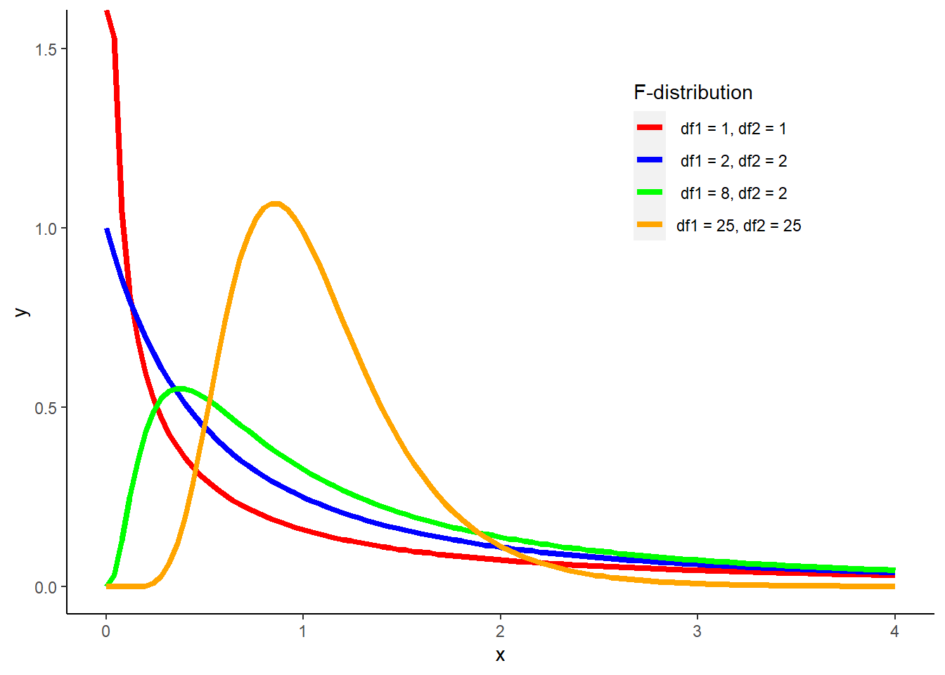
FIGURE 4.5: The F-distribution with varying degrees of freedom collected from two samples.
In practice, consider an F-distribution with 4 and 9 degrees of freedom. The upper-tail value from the \(F_{4,9}\) distribution so that the area under the curve to the right of it is 0.10 can be found with the qf() function:
qf(p = 0.90, df1 = 4, df2 = 9)## [1] 2.69268So, with 4 and 9 degrees of freedom, 10% of the area under the curve is greater than 2.69.
4.4.2 Two-sample F-test for variance
Assuming independent samples, our null hypothesis for the F-test for variances can be written as \(H_0: \sigma_1^2=\sigma_2^2\). Similar to a two-sample hypothesis for means, the following alternative hypotheses can be specified:
- \(H_A: \sigma_1^2<\sigma_2^2\)
- \(H_A: \sigma_1^2>\sigma_2^2\)
- \(H_A: \sigma_1^2\neq\sigma_2^2\)
We can assume the sample variance \(s_1^2\) estimates the population variance \(\sigma_1^2\) and similarly \(s_2^2\) estimates \(\sigma_2^2\). A test statistic \(F_0\) is then calculated using the ratio of these two values, that is:
\[F_0 = \frac{s_1^2}{s_2^2}\]
In R, the var.test() function performs an F-test to compare two variances. As an example, consider the data from the number of chirps that a striped ground cricket makes. These data are from the chirps data set used earlier in the chapter. Our goal is to test the hypothesis that the variances for the cps and cps_2 variables are equal at a level of significance of \(\alpha = 0.10\):
var.test(chirps$cps, chirps$cps_2, conf.level = 0.90)##
## F test to compare two variances
##
## data: chirps$cps and chirps$cps_2
## F = 0.83319, num df = 14, denom df = 14, p-value = 0.7375
## alternative hypothesis: true ratio of variances is not equal to 1
## 90 percent confidence interval:
## 0.3354586 2.0694086
## sample estimates:
## ratio of variances
## 0.8331872With a resulting p-value of 0.7375, we accept the null hypothesis and conclude that the variances for cps and cps_2 are equal. The ratio between variances of 0.8331 is close to 1, indicating the variances for both samples were similar. This result gives us confidence that we can use a pooled two-sample t-test that assumes equal variances between the two samples. It is a good practice to first conduct an F-test for variances and then conduct a two-sample t-test that either assumes the variances are equal (the pooled test) or not equal (the Welch test).
4.4.3 Exercises
4.8 Consider an F-distribution with the following upper-tail values and degrees of freedom. Use the qf() function to find the values of F that correspond to the parameters. What do you notice about the F values as the degrees of freedom and areas change?
- The area under the curve to the right of the value is 0.20 with 4 and 6 degrees of freedom.
- The area under the curve to the right of the value is 0.05 with 4 and 6 degrees of freedom.
- The area under the curve to the right of the value is 0.10 with 5 and 10 degrees of freedom.
- The area under the curve to the right of the value is 0.10 with 10 and 20 degrees of freedom.
4.9 For this next question, consider the intermediate and suppressed trees from the elm data set and your analyses from question 4.6.
- Perform an F-test comparing the variances for the heights (
HT) of intermediate and suppressed trees using a level of significance of \(\alpha = 0.05\). How would you interpret the results? - Perform an F-test comparing the variances for the diameters (
DIA) of intermediate and suppressed trees using a level of significance of \(\alpha = 0.10\) How would you interpret the results? - You will find a similar outcome for the hypothesis tests in the previous two questions. If you were interested in following up your analysis with a two-sample t-test of means, is a pooled or Welch t-test appropriate?
4.5 Summary
Statistical tests enable us to compare observed data with a claim whose truth we want to assess. We may be interested in seeing if a mean differs from a unique value (a one-sample t-test), if two independent means differ (a two-sample t-test), or if two dependent means differ (a paired t-test). We can also compare whether or not the variances from two samples differ. This can lead to a decision about which test for means is appropriate, i.e., a pooled or Welch t-test.
In these statistical tests, alternative hypotheses can be set up to be not equal to, less than, or greater than a specified value. The choice on how to set up the hypothesis test depends on the question being asked of the data. Two distributions were introduced in this chapter: the t-distribution and F-distribution. These distributions are widely used in other topics in statistics such as regression and analysis of variance, so it’s important to understand them as we’ll revisit them in future chapters.
4.6 References
Gelman, A. 2016. Why I prefer 50% rather than 95% intervals. Available at: https://statmodeling.stat.columbia.edu/2016/11/05/why-i-prefer-50-to-95-intervals/
Kloke, J., J.W. McKean. Nonparametric statistical methods using R. Chapman and Hall/CRC Press. 287 p.
Loon Preservation Committee. 1999. Mercury exposure as measured through abandoned common loon eggs in New Hampshire, 1998. Available at: https://www.fws.gov/newengland/PDF/contaminants/Contaminant-Studies-Files/Mercury-Exposure-as-Measured-through-Abandoned-Common-Loon-Eggs-in-New-Hampshire-1998-1999.pdf
Salsburg, D. 2001. The lady tasting tea: how statistics revolutionized science in the twentieth century. Holt Publishing. 340 p.
Wasserstein, R.L., and N.A. Lazar. 2016. The ASA statement on p-values: context, process, and purpose. The American Statistician 70(2): 129–133.