Chapter 13 Count regression
13.1 Introduction
Count data are widely collected and analyzed across natural resources disciplines, particularly in wildlife biology and conservation. Count data represent values from non-negative integers, e.g., 0, 1, 2, 3, etc. Values are obtained from counts rather than ranks such as in ordinal regression. Examples include the number of hazardous waste violations issued by an agency to a company, the counts of birds by ornithologists, and the number of butterfly species observed by a prairie researcher.
Models of count data require special consideration compared to other regression techniques presented in this book. Natural resources professionals also collect data on variables that exhibit zero-inflation (ZI), defined as an excess proportion of zeros relative to what would be expected under a given distribution. Count distributions such as the Poisson and negative binomial are useful in describing the stochastic nature of many variables. To quantify both structural and stochastic sources of variability, ZI count models are commonly employed.
13.2 Count data and their distributions
Count data represent discrete random variables given the nature of the data. The Poisson, binomial, and negative binomial distributions are commonly used distributions to reflect count data. The Poisson model is the benchmark model for count data, but it can be restrictive when estimating attributes other than the mean (Winkelmann 2008). The Poisson model is useful for describing events that are rare, independent, and collected from large populations. Its distribution is written as:
\[f_P(x) = \frac{\lambda^xe^{-\lambda}}{x!}\]
where \(x\) denotes a count of the number of occurrences (i.e., \(x = 0, 1, 2...\)} and \(\lambda\) represents the mean and variance of the distribution.
Negative binomial models are count models that are similar to Poisson models but include a dispersion parameter, making them more flexible and suitable for estimating a wide variety of count data. As this dispersion parameter increases, the variance of the distribution approaches the mean, making it similar to a Poisson distribution. In short, if the mean and variance are not equal to one another, dispersion is present, making for a useful case for employing the negative binomial distribution. A negative binomial probability can be obtained as a gamma mixture of Poisson distributions. If we consider \(x\) failures and \(r\) successes, the negative binomial is written as:
\[f_{NB}(x)={x+r-1\choose{r-1}}p^r(1-p)^x\] where \(p\) indicates the probability of success. Compared to the normal, these count distributions have a different appearance for the same set of parameters:
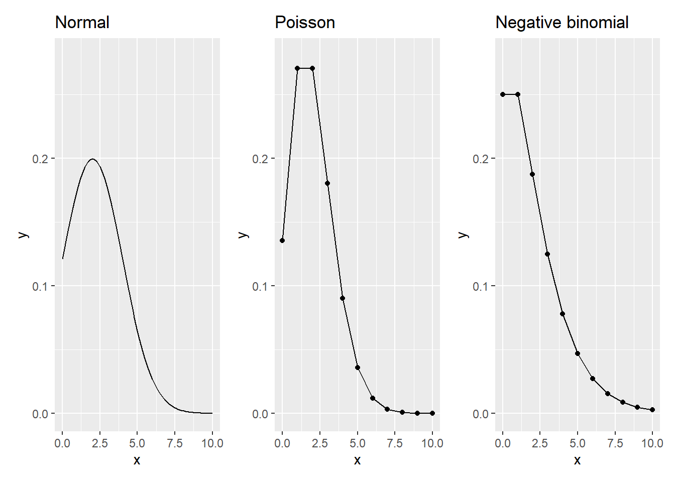
FIGURE 13.1: The normal, Poisson, and negative binomial distributions with a mean of 2 and variance of 2. (Dispersion parameter set to 0.5 for negative binomial.)
13.2.1 Case study: predicting fishing success
The fishing data set in the stats4nr package contains data on the number of fish caught by visitors to a state park. It includes the following variables:
livebait: whether or not the group used live bait (0/1),camper: whether or not the group brought a camper on their visit (0/1),persons: the number of people in the group,child: the number of children in the group, andcount: number of fish caught.
There are 250 observations in the data:
library(stats4nr)
fishing
## # A tibble: 250 x 6
## nofish livebait camper persons child count
## <dbl> <dbl> <dbl> <dbl> <dbl> <dbl>
## 1 1 0 0 1 0 0
## 2 0 1 1 1 0 0
## 3 0 1 0 1 0 0
## 4 0 1 1 2 1 0
## 5 0 1 0 1 0 1
## 6 0 1 1 4 2 0
## 7 0 1 0 3 1 0
## 8 0 1 0 4 3 0
## 9 1 0 1 3 2 0
## 10 0 1 1 1 0 1
## # ... with 240 more rowsHistograms work well for plotting count data such as the number of fish caught. We can see that most campers catch zero or only a few fish and only a few groups catch many fish, e.g., greater than 20:
ggplot(fishing, aes(x = count)) +
  geom_histogram() +
  labs (x = "Number of fish caught",
        y = "Number of occurences")
It is useful to quantify the mean and variance of the response variable to understand if dispersion is present:
mean(fishing$count)## [1] 3.296var(fishing$count)## [1] 135.3739In the case of the number of fish caught, we can say that overdispersion is present because the variance (135.4) is larger than the mean (3.3). Underdispersion would be present if the variance were less than the mean.
We are interested in predicting the number of fish caught using three predictor variables: the number of total people in the group, the number of children in the group, and whether or not the group used a camper during their visit. One might hypothesize that more people will increase the chances of fishing success, but more children, who are likely inexperienced and may not fish for long periods of time, may decrease the chances of fishing success. Similarly, groups that bring a camper for their visit may plan to camp for a longer duration, equating to more fishing time.
In R, the glm() function can be used to fit Poisson regression models to count data. The family = "poisson" statement within the function specifies a log link function in the model:
m.poisson <- glm(count ~ persons + child + camper,
                 family = "poisson", data = fishing)
summary(m.poisson)
##
## Call:
## glm(formula = count ~ persons + child + camper, family = "poisson",
## data = fishing)
##
## Deviance Residuals:
## Min 1Q Median 3Q Max
## -6.8096 -1.4431 -0.9060 -0.0406 16.1417
##
## Coefficients:
## Estimate Std. Error z value Pr(>|z|)
## (Intercept) -1.98183 0.15226 -13.02 <2e-16 ***
## persons 1.09126 0.03926 27.80 <2e-16 ***
## child -1.68996 0.08099 -20.87 <2e-16 ***
## camper 0.93094 0.08909 10.45 <2e-16 ***
## ---
## Signif. codes: 0 '***' 0.001 '**' 0.01 '*' 0.05 '.' 0.1 ' ' 1
##
## (Dispersion parameter for poisson family taken to be 1)
##
## Null deviance: 2958.4 on 249 degrees of freedom
## Residual deviance: 1337.1 on 246 degrees of freedom
## AIC: 1682.1
##
## Number of Fisher Scoring iterations: 6The scale and magnitude of the coefficients confirm our hypotheses about the predictor variables and their relationship with fishing success. In addition to the output from the coefficients, also of note is the AIC value, a useful metric that can be compared to models fit with other distributions.
For fitting negative binomial regressions in R, the glm.nb() function available in the MASS package (Venables and Ripley 2002) is flexible. We can fit a similar model form as the Poisson, but instead relying on the dispersion parameter inherent to the negative binomial distribution:
library(MASS)

m.nb<- glm.nb(count ~ persons + child + camper,
              data = fishing)
summary(m.nb)
##
## Call:
## glm.nb(formula = count ~ persons + child + camper, data = fishing,
## init.theta = 0.4635287626, link = log)
##
## Deviance Residuals:
## Min 1Q Median 3Q Max
## -1.6673 -0.9599 -0.6590 -0.0319 4.9433
##
## Coefficients:
## Estimate Std. Error z value Pr(>|z|)
## (Intercept) -1.6250 0.3304 -4.918 8.74e-07 ***
## persons 1.0608 0.1144 9.273 < 2e-16 ***
## child -1.7805 0.1850 -9.623 < 2e-16 ***
## camper 0.6211 0.2348 2.645 0.00816 **
## ---
## Signif. codes: 0 '***' 0.001 '**' 0.01 '*' 0.05 '.' 0.1 ' ' 1
##
## (Dispersion parameter for Negative Binomial(0.4635) family taken to be 1)
##
## Null deviance: 394.25 on 249 degrees of freedom
## Residual deviance: 210.65 on 246 degrees of freedom
## AIC: 820.44
##
## Number of Fisher Scoring iterations: 1
##
##
## Theta: 0.4635
## Std. Err.: 0.0712
##
## 2 x log-likelihood: -810.4440Note that the scale and magnitude of the coefficients between the Poisson and NB models are similar, but with slightly different values. The dispersion parameter Theta is 0.4635 with a standard error of 0.0712.
We can also plot the predictions of number of fish caught from the Poisson and negative binomial models by applying the m.poisson and m.nb models to the new.fish data set. Specifying type = "response" provides the predicted number of fish caught:
new.fish <- tibble(
  persons = c(1, 2, 3, 4, 1, 2, 3, 4),
  child = c(0, 0, 0, 0, 0, 0, 0, 0),
  camper = c(0, 0, 0, 0, 1, 1, 1, 1))
new.fish <- new.fish %>%
mutate(count_p_pred = predict(m.poisson,
newdata = new.fish,
type = "response"),
count_nb_pred = predict(m.nb,
newdata = new.fish,
type = "response"))We can see that as the number of people in a group increases, so too does the number of fish caught. The Poisson model predicts a greater number of fish caught for groups that visit state parks with a camper, while for groups without a camper the negative binomial model predicts a greater number of fish caught:
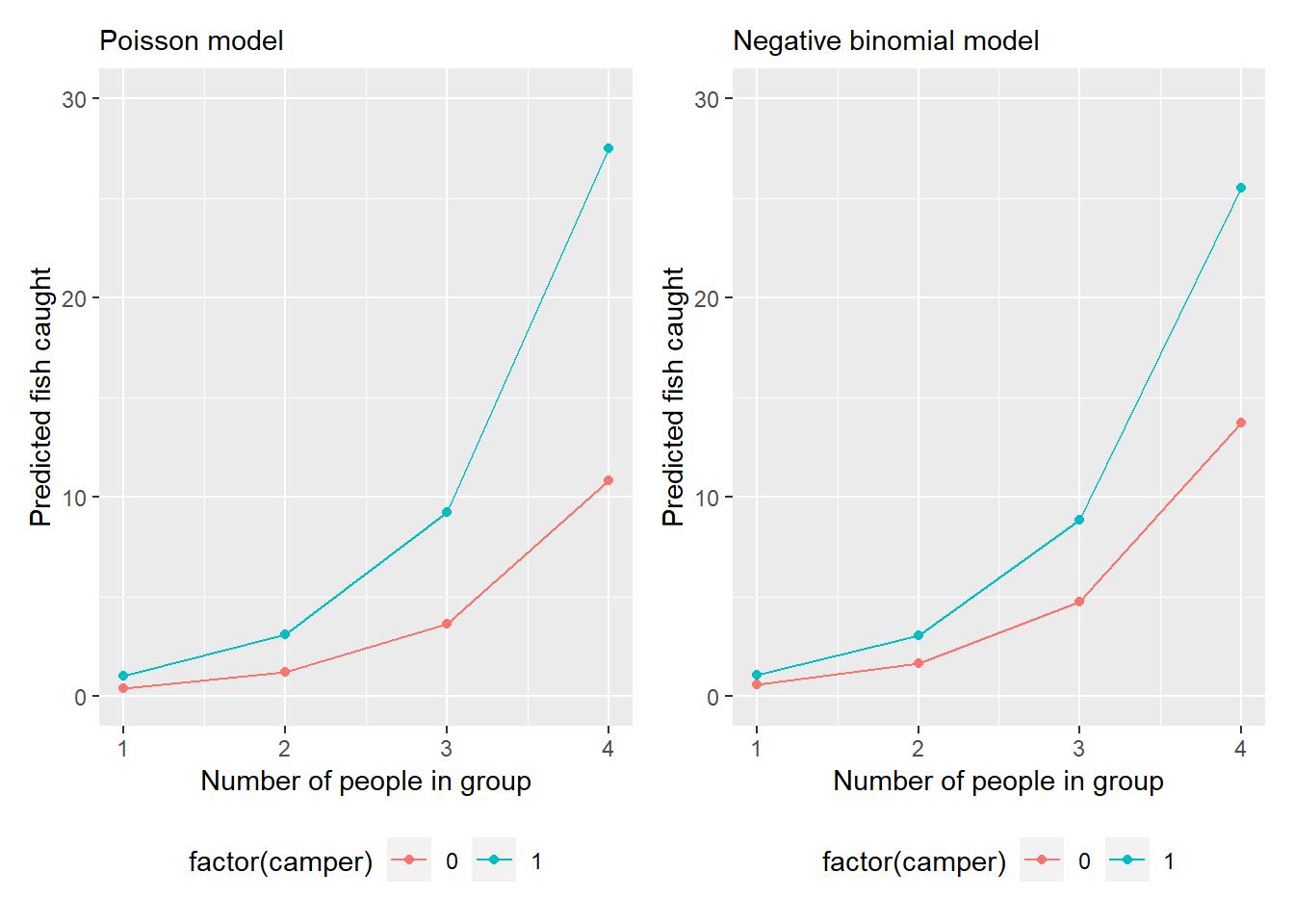
FIGURE 13.2: Model predictions of number of fish caught from the fishing data set.)
13.2.2 Exercises
13.1 You hypothesize that as forests become older, their canopies become dominated by only a few species, which limits light availability for other species growing in the understory. Data to examine this hypothesis were acquired from the Hubachek Wilderness Research Center, an experimental forest located in northern Minnesota (Gill et al. 2019). Data were collected from 36 forest inventory plots with at least one tree larger than 12.7 cm in diameter. The number of species (num_spp), number of standing dead trees (num_dead), and average height of the trees in the plot (ht_m; meters) are the variables of interest.
- Run the code below to create the data set sp_ht to use in this analysis. Does the count variable of interest (
num_spp) display characteristics of underdispersion or overdispersion? Comment on the usefulness of using the Poisson distribution for this variable.
sp_ht <- tibble(
  num_spp = c(4, 3, 2, 4, 2, 4, 2, 3, 2, 2,
              5, 1, 7, 4, 4, 7, 4, 6, 4, 5,
              3, 5, 5, 3, 7, 2, 5, 5, 3, 5,
              3, 5, 2, 4, 5, 4),
  num_dead= c(1, 1, 0, 0, 1, 0, 1, 1, 0, 0,
              2, 0, 0, 3, 0, 0, 0, 0, 0, 0,
              0, 0, 0, 0, 1, 0, 1, 0, 0, 0,
              0, 2, 0, 0, 0, 0),
  ht_m = c(17.6, 19.8, 26.0, 17.4, 19.8, 20.7,
           14.7, 17.6, 11.6, 19.4, 12.7, 16.4,
           12.6, 17.9, 23.2, 14.5, 18.6, 15.0,
           11.5, 15.1, 13.8, 9.9, 20.2, 7.3,
           6.2, 11.4, 16.5, 8.7, 9.8, 6.9,
           18.0, 10.0, 12.8, 13.7, 12.8, 16.7)
  )
Create a histogram for the
num_sppvariable and comment on its distribution.Fit two count regression models predicting the number of species in a plot based on its average height. One model should assume the Poisson and the other a negative model distribution. Based on their AIC values, which model would you prefer and why?
13.2 Use the Poisson regression model you created in question 13.1 to make a prediction of the number of species for five additional forest inventory plots with mean heights of 12, 13, 19, 21, and 24 meters.
13.3 Make a graph using ggplot() that fits the Poisson model you created in question 13.1. For a range of tree heights from 5 to 30 meters along the x-axis, plot the predictions of the number of species for the model on the y-axis.
13.3 Zero-inflated models
To account for data with a high proportion of zeros, zero-modified count models, or zero-inflated models are often applied. For example, you may visit a forest to count the number of warblers you observe, but on repeated visits you observe none. Zero inflation is also apparent in the fishing data set, as the histogram indicates that zero is the most common value (i.e., the mode) for number of fish caught. These data result in excess zeros which make modeling with standard regression techniques a challenge.
In addition to visualizing them, calculating the percent of observations with zero as the response variable can help inform whether or not zero-inflated models should be considered. There are no guidelines or statistical tests that evaluate the specific number of observations required to perform zero-inflated regression. However, a general rule of thumb with natural resources data is that if 25% or more of your observations of a response variable are zero, zero-inflated models should be evaluated.
If the number of different response variable counts are relatively small (i.e., less than 30), summarizing the percent of observation by each count response can be done with the summarize() function. For the fishing data set, we calculate that 56.8% of the fishing groups caught zero fish:
fishing %>%
  group_by(count) %>%
  summarize(num_fish = n()) %>%
  mutate(Pct = num_fish / sum(num_fish) * 100)
## # A tibble: 25 x 3
## count num_fish Pct
## <dbl> <int> <dbl>
## 1 0 142 56.8
## 2 1 31 12.4
## 3 2 20 8
## 4 3 12 4.8
## 5 4 6 2.4
## 6 5 10 4
## 7 6 4 1.6
## 8 7 3 1.2
## 9 8 2 0.8
## 10 9 2 0.8
## # ... with 15 more rowsZero-inflated models estimate two equations: a count model and a model describing the excess zeros. From these kinds of models, zero-inflated Poisson (ZIP) and zero-inflated negative binomial (ZINB) models are two types of models that estimate structural and stochastic zeros (Welsh et al. 1996; Gray 2005). In the ZIP model, zero counts are estimated by those derived from a binomial or Poisson distribution. Thus, the ZIP model has two parts: a Poisson count model and a logit model for predicting the excess zeros. A ZIP probability is estimated by:
\[ f_{ZIP}(x) = \left\{ \begin{array}{ll} \pi + (1-\pi)\mbox{e}^{-\lambda}, x = 0 \\ (1-\pi)f_P(x), x = 1, 2, 3, ... \end{array} \right. \]
where \(\pi\) is the probability of zero occurrence, \(\lambda\) is estimated using independent variables, and \(f_{P}(y)\) is the Poisson distribution.
Similar to the NB distribution, a ZINB distribution includes a dispersion parameter \(\alpha\). A ZINB probability is estimated by the mass function:
\[ f_{ZINB}(x) = \left\{ \begin{array}{ll} \pi + (1-\pi)(\frac{1}{1+\lambda\alpha})^{1/\alpha}, x = 0 \\ (1-\pi)f_{NB}(x), x = 1, 2, 3, ... \end{array} \right. \]
where \(\alpha\) is the dispersion parameter and \(f_{NB}(y)\) is the negative binomial distribution.
Rather than modeling the excess zeros directly, some modelers will transform the data instead. After transforming a variable of interest, you could run a general linear model, however, the response variable will change. This will not necessarily improve linearity or assist the model meeting the assumption of homogeneity of variance. Furthermore, transformation of data with excess zeros cannot be accomplished with popular methods such as the logarithmic or reciprocal transformation.
13.3.1 Fitting zero-inflated models in R
The pscl package, abbreviated for the Political Science Computational Laboratory at Stanford University, fits a suite of models used in political science applications, including count models. The package is widely used to fit zero-inflated models. We can install and load the package to use it:
install.packages("pscl")
library(pscl)
The zeroinfl() function fits ZIP and ZINB models using syntax that is similar to the glm() function. By default, the zeroinfl() function will assume you wish to fit a ZIP model, which we can do with the fishing data:
m.zip <- zeroinfl(count ~ persons + child + camper,
                  data = fishing)
summary(m.zip)
##
## Call:
## zeroinfl(formula = count ~ persons + child + camper, data = fishing)
##
## Pearson residuals:
## Min 1Q Median 3Q Max
## -3.05440 -0.74336 -0.44275 -0.07559 27.99304
##
## Count model coefficients (poisson with log link):
## Estimate Std. Error z value Pr(>|z|)
## (Intercept) -0.79826 0.17081 -4.673 2.96e-06 ***
## persons 0.82904 0.04395 18.862 < 2e-16 ***
## child -1.13666 0.09299 -12.224 < 2e-16 ***
## camper 0.72425 0.09314 7.776 7.51e-15 ***
##
## Zero-inflation model coefficients (binomial with logit link):
## Estimate Std. Error z value Pr(>|z|)
## (Intercept) 1.6636 0.5155 3.227 0.00125 **
## persons -0.9228 0.1992 -4.632 3.62e-06 ***
## child 1.9046 0.3261 5.840 5.21e-09 ***
## camper -0.8336 0.3527 -2.364 0.01808 *
## ---
## Signif. codes: 0 '***' 0.001 '**' 0.01 '*' 0.05 '.' 0.1 ' ' 1
##
## Number of iterations in BFGS optimization: 12
## Log-likelihood: -752.7 on 8 DfThe primary item of note here is that two sets of coefficients are provided in the output: the first for the count model and the second for the zero inflation model. The count model coefficients for the ZIP model would be analogous to the coefficients found in the standard Poisson model (m.poisson) above.
The zero-inflated model coefficients are similar to a logistic regression as they are fit with the logit link function and address the question of whether the group caught zero fish or not. The signs of the coefficients for the zero-inflated model are opposite from the count model. This makes intuitive sense. For example, the persons coefficient in the count model (0.82904) indicates more people in a fishing group would catch more fish and the persons coefficient in the zero-inflated model (-0.9228) indicates more people in a fishing group would lower the probability of catching zero fish.
A ZINB model can be fit by setting the distribution to "negbin" in the zeroinfl() function:
m.zinb <- zeroinfl(count ~ persons + child + camper,
                   dist = "negbin", data = fishing)
summary(m.zinb)
##
## Call:
## zeroinfl(formula = count ~ persons + child + camper, data = fishing,
## dist = "negbin")
##
## Pearson residuals:
## Min 1Q Median 3Q Max
## -0.71806 -0.56103 -0.38173 0.04398 16.16365
##
## Count model coefficients (negbin with log link):
## Estimate Std. Error z value Pr(>|z|)
## (Intercept) -1.6178 0.3202 -5.052 4.36e-07 ***
## persons 1.0901 0.1117 9.761 < 2e-16 ***
## child -1.2613 0.2473 -5.100 3.40e-07 ***
## camper 0.3857 0.2461 1.567 0.117108
## Log(theta) -0.5929 0.1580 -3.753 0.000174 ***
##
## Zero-inflation model coefficients (binomial with logit link):
## Estimate Std. Error z value Pr(>|z|)
## (Intercept) -12.0956 67.7886 -0.178 0.858
## persons 0.2906 0.7315 0.397 0.691
## child 11.0538 67.7088 0.163 0.870
## camper -10.8729 67.7236 -0.161 0.872
## ---
## Signif. codes: 0 '***' 0.001 '**' 0.01 '*' 0.05 '.' 0.1 ' ' 1
##
## Theta = 0.5527
## Number of iterations in BFGS optimization: 44
## Log-likelihood: -395.5 on 9 DfNote the similarity and differences between the ZIP and ZINB coefficients in the R output. The primary addition to the ZINB output is the dispersion parameter Theta = 0.5527. When implementing the zero-inflation model coefficients to make predictions on new data, a threshold or cutpoint probability needs to be specified to determine if a zero or non-zero prediction results. For this a standard 0.50 or 0.75 probability is often specified.
13.3.2 Exercises
13.4 The choice of which count regression model to implement depends in part on the characteristics of the response variable. Write R code and describe whether the following variables represent overdispersion, underdispersion, or equal dispersion. Also comment on which modeling technique may be appropriate for the data (e.g., Poisson, negative binomial, zero-inflated Poisson, or zero-inflated negative binomial).
- Ant species richness (
spprich) in bogs and forests in New England, USA (available in the ants data set from the stats4nr package). - The number of birds (
NumBirds) observed in west-central California suburbs (available in the birds data set from the stats4nr package). - The number of tree species (
num_spp) observed in forest inventory plots in an experimental forest in Minnesota (available from question 13.1). - The number of standing dead trees (
num_dead) observed in forest inventory plots in an experimental forest in Minnesota (available from question 13.1).
13.5 Compare the Akaike’s information criterion (AIC) for the zero-inflated Poisson and zero-inflated negative binomial models fit to the fishing data set. Which model is of better quality and why do you suspect the degrees of freedom differ between the two models?

FIGURE 13.3: An American marten. Image: Bailey Parsons, Wikimedia Commons.
13.6 A large number of standing dead trees in a forest is an indicator of quality habitat to sustain populations of American marten (Martes americana), a mammal species found in northern temperate and boreal forests. Using the data set provided from the experimental forest in question 13.1, answer the following questions.
- Write R code to determine the percentage of forest inventory plots that contain no observations of standing dead trees.
- Fit a model that predicts the number of standing dead trees (
num_dead) in a forest plot using the average height of trees in a stand (ht_m). Fit a standard Poisson and zero-inflated Poisson model and compare them with AIC. Which model would you prefer?
13.4 Evaluating count regression models
While AIC is a useful metric to compare multiple count regression models (e.g., the Poisson, NB, ZIP, and NINB models), a number of other useful measures can determine the uncertainty and goodness of fit for count models. Diagnostic plots that display differences between predicted and observed counts are often employed to examine model fit of count regression models. Diagnostic plots can visualize the deviance residuals, showing trends in overestimations or underestimations across a range of values. Similarly, Pearson’s residuals rely on the chi-square (\(\chi^2\)) distribution and can be used to assess model fit. As an example, we can visualize the residual values from our model fit with a Poisson distribution and store them in the fishing data set. We first predict the number of fish and then determine the deviance and Pearson’s residuals by changing the type = statement within the resid() function:
fishing <- fishing %>%
  mutate(count_pred = predict(m.poisson,
                              newdata = fishing,
                              type = "response"),
         res_dev = resid(m.poisson, type = "deviance"),
         res_pear = resid(m.poisson, type = "pearson"))
Then, we can plot the two residual values to determine trends and assess model fit:
ggplot(fishing, aes(count_pred, res_dev)) +
  geom_point() +
  labs(x = "Fitted value",
       y = "Deviance residual")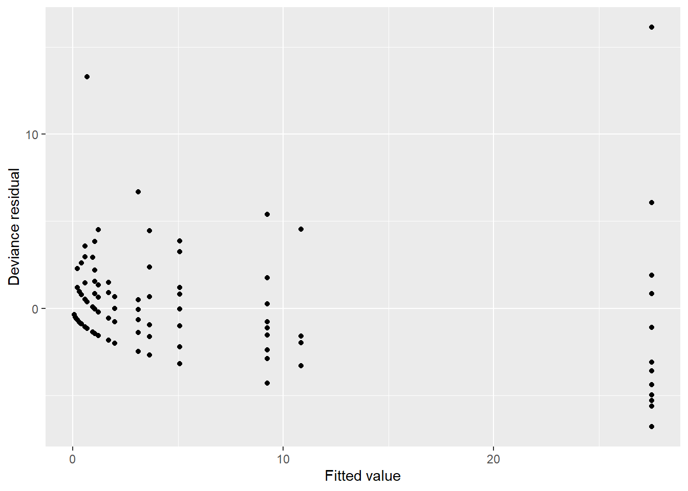
ggplot(fishing, aes(count_pred, res_pear)) +
  geom_point() +
  labs(x = "Fitted value",
       y = "Pearson residual")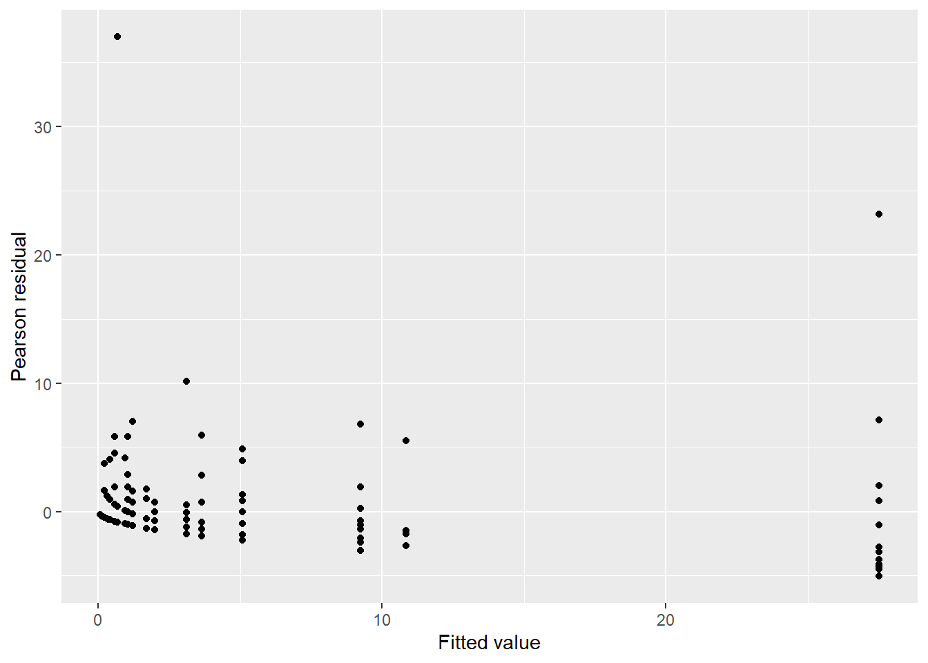
There is some concern with a single data point with a small estimated mean with a large residual (e.g., Pearson residual greater than 30 fish caught). The characteristics of this data point are worth looking into with more detail.
The root mean square error (RMSE) and mean bias (MB) are two metrics that allow you to determine the uncertainty of model predictions:
\[ RMSE = \sqrt{\sum_{i=1}^{n}{(y_i-\hat{y}_i)^2/n}} \]
\[ MB = \sum_{i=1}^{n}{(y_i-\hat{y}_i)/n} \]
where \(y_i\) is the observed count, \(\hat{y}_i\) is the estimated count, and \(n\) is the number of observations.
Pearson’s chi-square (\(\chi^2\)) statistic is a commonly used metric used to determine goodness of fit with count regression models.
\[ \chi^2 = \sum_{i=1}^{n}\frac{(y_i-E({y_i}))^2}{Var({y_i})} \] The expected value \(E({y_i})\) and variance \(Var({y_i})\) can be calculated for the response variable of interest depending on the count model (e.g., Poisson, NB, ZIP, or ZINB; Zuur et al. [2009]). Using the (\(\chi^2\)) statistic, data can be divided into intervals and the numbers of observations within each interval can be compared. Generally, a satisfactory model fit is indicated if the ratio of the \(\chi^2\) to its degrees of freedom is close to one.
13.4.1 Exercises
13.7 Create a diagnostic plot using ggplot() that shows the Pearson residuals for the zero-inflated Poisson model that predicts the number of fish caught from the fishing data set.
13.8 Write two functions in R that can be applied to any data set with observations and model predictions. One function should calculate the root mean square error (RMSE) and the other the mean bias (MB). Use the functions to determine the RMSE and MB for the standard Poisson and zero-inflated Poisson models that predict the number of fish caught from the fishing data set.
13.5 Summary
Count data, where observations represent non-negative integers, are widely found across natural resources disciplines. The Poisson distribution is the classic count distribution that can describe many distributions of count data. While it assumes that a mean value is equal to its variance, if this assumption cannot hold, consider if the data are distributed as a negative binomial distribution. When modeling data with a negative binomial, a dispersion parameter is specified to account for differences in values for the mean and variance. If a number of excess zeros are present in the data, consider the zero-inflated implementations of these models. Zero-inflated models estimate two equations: one that reflects the count model (analogous to the standard Poisson or negative binomial models) and another that estimates a logistic model for predicting the excess zeros.
Count models are generalized linear models and can be fit in R using code and syntax similar to logistic regression. The glm() function can fit standard Poisson models while the glm.nb() function from the MASS package fits negative binomial models. The pscl package is popular for fitting zero-inflated versions of these models and provides parsimonious output for interpreting and assessing models. It is a good practice to fit different versions of count models, including standard and zero-inflated ones, and compare their performance with metrics such as AIC and root mean square error and visualizations such as diagnostic plots. Having a thorough understanding of these regression modeling techniques will aid you when you encounter count data.
13.6 References
Gill, K.G., L.B. Johnson, R.A. Olesiak, R.J. Prange, and A.J. David. 2019. Defining the University of Minnesota experimental forests landbase. Retrieved from the University of Minnesota Digital Conservancy. Available at: https://hdl.handle.net/11299/209141.
Gray, B.R. 2005. Selecting a distributional assumption for modelling relative densities of benthic macroinvertebrates. Ecological Modelling 185: 1-–12.
Venables, W. N., and B.D. Ripley. 2002. Modern applied statistics with S. Fourth edition. Springer, New York.
Welsh, A.H., R.B. Cunningham, C.F. Donnelly, and D.B. Lindenmayer. 1996. Modelling the abundance of rare species: statistical models for counts with extra zeros. Ecological Modelling 88: 297-–308.
Winkelmann, R. 2008. Econometric analysis of count data. Springer, Berlin.
Zuur, A., E.N. Ieno, N. Walker, A.A. Saveliev, G.M. Smith, G.M. 2009. Mixed effects models and extensions in ecology with R. Springer-Verlag, New York.