Chapter 11 Analysis of covariance
11.1 Introduction
Analysis of variance tests whether several populations have the same means by comparing how far apart they are and how much variation there is within a sample. Linear regression allows us to examine relationships between at least two quantitative variables. Analysis of covariance (ANCOVA) is a general linear model which blends concepts from ANOVA and regression. The ANCOVA technique evaluates whether the means of a dependent variable are equal across levels of a categorical independent variable, often a treatment that is controlled in an experiment or some other factor variable. The ANOVA process controls for the effects of other continuous variables that are not of primary interest, known as covariates.
This chapter will discuss how ANCOVA combines principles from ANOVA and regression, the assumptions of an ANCOVA model and how they can be assessed, and how to apply ANCOVA techniques to natural resources data sets.
11.2 Analysis of covariance
You can think about ANCOVA as an application when we add a continuous covariate in an ANOVA analysis. These covariates are not generally a part of the manipulation of an experiment, but they may have an influence on the dependent variable. In natural resources, common covariates include elements of time (e.g., number of years since a disturbance to a forest or number of days a plant was subject to drought stress) or initial conditions prior to an event (e.g., the density of a forest prior a disturbance or the size of a plant prior to being exposed to drought stress). In ANCOVA, the covariate can be treated as it might be in a regression equation:
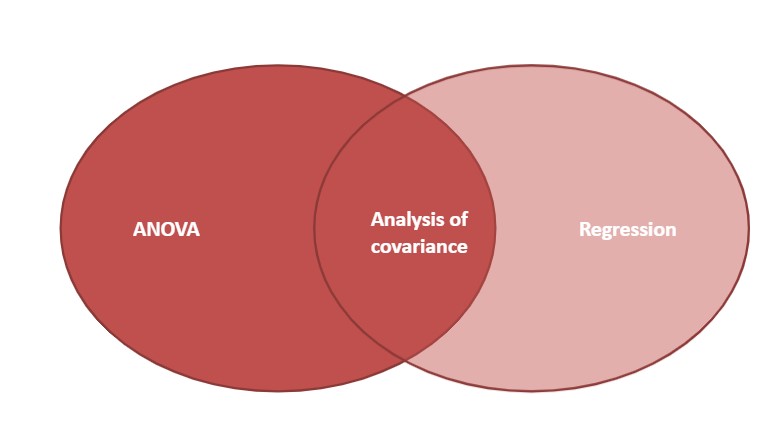
FIGURE 11.1: Analysis of covariance blends analysis of variance and regression.
The ANCOVA model takes the form:
\[ y_{ij}= \mu + \tau_{i}+ \textbf{B}(x_{ij}-\bar{x}_i)+\varepsilon_{ij}\] where,
- \(y_{ij}\) is the jth observation mean from the ith level,
- \(\mu\) is the overall mean,
- \(\tau_{i}\) is the effect of the ith level of the treatment,
- \(x_{ij}\) is the jth observation of the covariate in the ith level,
- \(\bar{x}_i\) is the ith group mean, and
- \(\varepsilon_{ij}\) is the random error term.
Like any statistical test, there are several key assumptions that underlie the use of ANCOVA and affect the interpretation of the results. The assumptions used in linear regression and ANOVA also hold for ANCOVA analyses, i.e., the treatment effect and the covariate are independent, the variance is homogeneous, there is a linear relationship between the covariate and response variable, and residuals (errors) are normally distributed. For ANCOVA, an added assumption is that the regression slopes are the same for all treatment groups.
11.2.1 Testing equality of slopes in ANCOVA
If an assumption is that the slope of the covariate is equal across all treatment groups, it needs to be assessed prior to reporting the results from an ANCOVA. After plotting the data using scatter plots and line graphs, you can visually compare if slopes are equal:
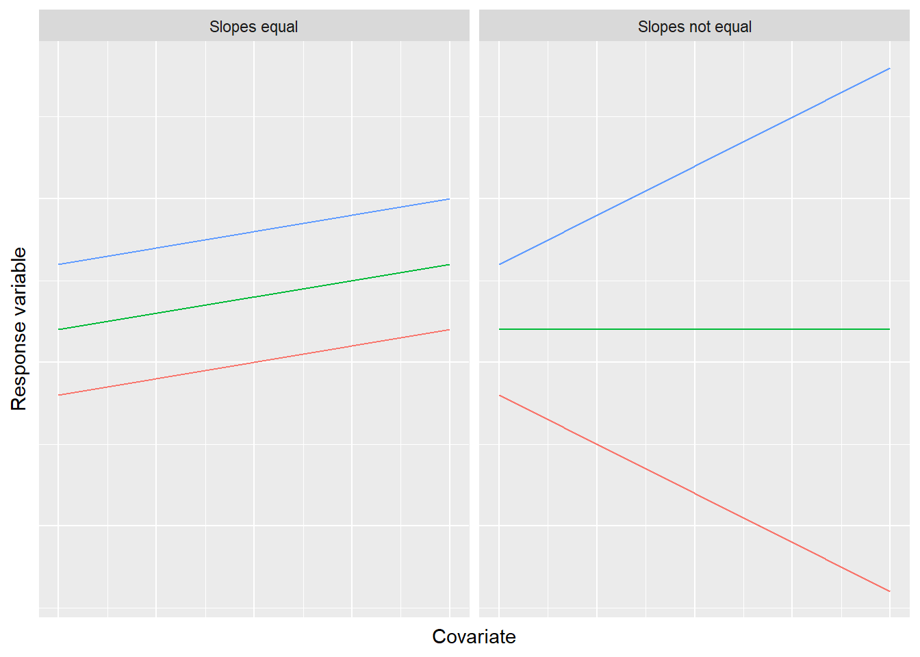
FIGURE 11.2: An assumption of the analysis of covariance is the equality of slopes across the range of values for the covariate.
As an example, consider the fish data set from the stats4nr package (Puranen 1917). Here, we can consider the species of fish as a factor and the length of the fish (Length1) as a covariate. We might be interested in predicting the weight of a fish (Weight) using these two variables. For simplicity, we’ll create a data set that contains observations for two species: bream and pike:
library(stats4nr)

fish <- fish %>%
  filter(Species %in% c("Bream", "Pike"))
We can plot the data to see the weight-length differences between the two species:
p.fish <- ggplot(fish, aes(Length1, Weight, col = Species)) +
  geom_point() +
  stat_smooth(method = "lm")
p.fish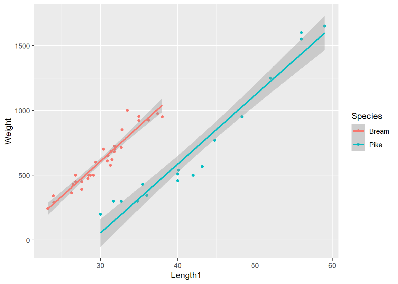
Can we make the claim that the two slopes are equal? Note that although the range of length measurements for pike is greater than for bream, for a given length of a fish, bream will weigh more than pike. For the ANCOVA analysis, our key interest lies in assessing the slopes of the two lines.
An appropriate statistical test to examine the equality of slopes is a t-test. The test statistic can be computed as:
\[ t = \frac{\beta_{\mbox{1, bream}}-\beta_{\mbox{1, pike}}}{\sqrt{(SE_{bream}^2+SE_{pike}^2)}}\] where \(\beta_{\mbox{1,i}}\) is the slope regression coefficient and \(SE_i\) is the standard error for the slope for each species.
We can fit two regressions to the bream and pike data simultaneously using a group_by statement. Then, the tidy() function from the broom package can return the regression coefficients and standard errors:
library(broom)

fish_spp <- group_by(fish, Species)

fish.coef <- do(fish_spp,
   tidy(lm(Weight ~ Length1, data = .)))

fish.coef
## # A tibble: 4 x 6
## # Groups: Species [2]
## Species term estimate std.error statistic p.value
## <chr> <chr> <dbl> <dbl> <dbl> <dbl>
## 1 Bream (Intercept) -1015. 91.2 -11.1 1.54e-12
## 2 Bream Length1 54.1 2.99 18.1 2.18e-18
## 3 Pike (Intercept) -1541. 144. -10.7 2.04e- 8
## 4 Pike Length1 53.2 3.32 16.0 7.65e-11Note the slope estimate for bream is 54.1 and the slope estimate for pike is 53.2. With the null hypothesis \(H_0: \beta_{1, bream} = \beta_{1, pike}\) and the alternative hypothesis \(H_1: \beta_{1, bream} \ne \beta_{1, pike}\), the t-statistic can be computed as:
\[ t = \frac{54.1-53.2}{\sqrt{2.99^2+3.32^2}} = \frac{0.90}{4.47} = 0.201\]
With such a small value of t, we can logically accept the null hypothesis and conclude that the two slopes are equal. Performing the t-test by hand would be an approach to use if all that was available were the values of the estimates and their standard errors. Another way to test if the slopes are equal in R is to following this process:
- Fit a “full” model with an interaction effect to examine if the effect of fish length on weight depends on species. (This is the definition of an interaction.)
- Fit a “reduced” model without an interaction effect.
For the fish data, the models can be written as:
fish.full <- lm(Weight ~ Length1 * Species, data = fish)

fish.reduced <- lm(Weight ~ Length1 + Species, data = fish)
Two R objects can be added to an anova() statement to examine the null hypothesis that the slopes are equal:
anova(fish.full, fish.reduced)## Analysis of Variance Table
##
## Model 1: Weight ~ Length1 * Species
## Model 2: Weight ~ Length1 + Species
## Res.Df RSS Df Sum of Sq F Pr(>F)
## 1 47 340835
## 2 48 341108 -1 -273.33 0.0377 0.8469Similar to what was observed when manually calculating the t-statistic, we observe a large p-value (0.8469) comparing the two models, indicating the effect of fish length on weight does not depend on species. Hence, we can conclude with our data of bream and pike observations that we can perform ANCOVA procedures because the slopes are equal for each species across the range of the covariate Length1.
11.2.2 ANCOVA hypothesis tests and outcomes
Hypothesis tests for the ANCOVA model are very similar to an ANOVA, but the key difference is that the population means for each treatment t are adjusted for the covariate. For example, we can label the population mean of the first factor level as \(\mu_1^*\). The null and alternative hypotheses can be written as
\[H_0 = \mu_1^* = \mu_2^* = ... = \mu_t^*\]
\[H_A = \mu_i^* \ne \mu_j^*, \mbox{for some } i \ne j\]
The variance can be partitioned in an ANCOVA model by examining three components:
The treatment effect reflects the main treatment effect or factor in the study, e.g., the species of fish.
The covariate effect adjusts the sums of squares for the covariate, i.e., the length of the fish.
The error represents the sum of squares within each treatment group.
You can see both elements of ANOVA and regression in the ANCOVA model. The “regression” component is represented by the covariate and the “ANOVA” part is represented by the treatment. Of course, there will also be error in our model that cannot be explained by the treatment or covariate.
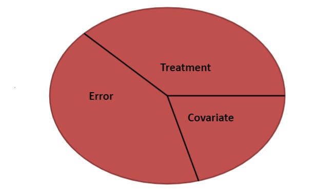
FIGURE 11.3: Variance partitioning in analysis of covariance.
We can use the ANCOVA table to make inference about the factors of interest and the covariate. Note how we can carry out two hypothesis tests with ANCOVA: one for the covariate and one for the treatment effect (as noted in the two F-statistics we calculate).
| Source | Degrees of freedom | Sums of squares | Mean square | F |
|---|---|---|---|---|
| Covariate | 1 | SS(Cov) | MS(Cov) = SS(Cov) | MS(Cov) / MSW |
| Treatment | k-1 | SS(B) | MSB = SSB / k-1 | MSB / MSW |
| Error (Within) | n-k-1 | SSW | MSW = SSW / n-k-1 |
|
| Total | n-1 | TSS |
|
|
Similar to ANOVA, multiple comparisons can be performed on the treatment effect within an ANCOVA model. Given we already know there are differences between the weights of bream and pike fish, the LSD.test() function from the agricolae package provides different letters denoting significant differences between the two species:
library(agricolae)

lsd.fish <- LSD.test(fish.reduced, "Species", p.adj = "bonferroni")
lsd.fish
## $statistics
## MSerror Df Mean CV
## 7106.423 48 656.902 12.8329
##
## $parameters
## test p.ajusted name.t ntr alpha
## Fisher-LSD bonferroni Species 2 0.05
##
## $means
## Weight std r LCL UCL Min Max Q25 Q50
## Bream 626.0000 206.6046 34 596.9317 655.0683 242 1000 481.25 615
## Pike 718.7059 494.1408 17 677.5971 759.8146 200 1650 345.00 510
## Q75
## Bream 718.5
## Pike 950.0
##
## $comparison
## NULL
##
## $groups
## Weight groups
## Pike 718.7059 a
## Bream 626.0000 b
##
## attr(,"class")
## [1] "group"With a mean of 719 and 626 grams for pike and bream, respectively, we find there are significant differences between the weights of the two species after adjusting for the covariate Length1. In terms of the consequences of outcomes, the addition of the covariate in ANCOVA reduces the probability of Type II error, i.e., failing to reject the null hypothesis when the null hypothesis is false.
11.2.3 Exercises
11.1 Make a bar plot showing the fish weight results presented earlier in this chapter.
- Write code in
ggplot()that displays two bars that show the mean fish weight for bream and pike. For error bars, present the 95% confidence limits for mean weights. (HINT: Assume a value t of 1.96 in your calculation.) Add letters denoting significant differences above the bar plots between the two species. - What interesting finding do you observe comparing the bar plot you created with the ANOVA output?
11.2 Perform ANCOVA on the entire fish data set, i.e., on all seven species and 157 observations. Using these data, evaluate whether or not you meet the assumptions of ANCOVA and report your results.
11.3 Perform an ANCOVA using Loblolly, a data set built into R. The data set contains the height, age, and seed source of loblolly pine (Pinus taeda) trees.
- Create a scatter plot of
age(x-axis) andheight(y-axis), adding color and a linear regression line (without confidence intervals) for each seed source (Seed). - Write code to evaluate the assumptions of whether or not an ANCOVA can be performed to determine loblolly pine tree height using seed source as a factor and age as a covariate.
- Summarize the ANCOVA results using a statistical test at \(\alpha = 0.10\). Do specific seed sources produce taller heights of loblolly pine trees?
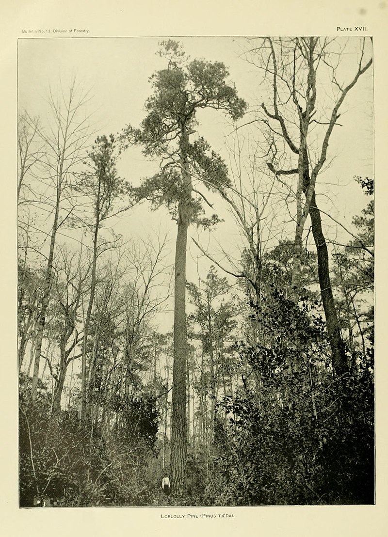
FIGURE 11.4: An old-growth loblolly pine tree. Image: Wikimedia Commons
11.3 Summary
Analysis of covariance blends components of linear regression and analysis of variance by integrating a quantitative covariate and a categorical treatment variable. The primary difference between an ANOVA and an ANCOVA model is the addition of the continuous covariate. An analyst should select an appropriate covariate that explains a portion of the variability in the dependent variable of interest. A key step in performing an ANCOVA analysis is to first determine the equality of slopes when investigating the covariate-response variable relationship at different levels of the treatment or factor variable. The ANCOVA adjusts each treatment mean based on the dependent variable.
You may encounter obstacles when performing an ANCOVA. For example, what if the slopes are examined and the results are that they are not equal? In this case, you have three options for moving forward with your analysis. First, consider dropping the covariate and running a one-way ANOVA. Second, consider “categorizing” the covariate and running a two-way ANOVA. As an example, if slopes were not equal in the fish data set, we might have created an indicator variable that labeled them as long and short fish, using a threshold value for length that we deem appropriate. Lastly, you could retain the covariate and consider fitting a general linear model. In the event that you have several covariates that are a part of a data set, consider multiple regression techniques.
11.4 References
Puranen, J. 1917. Fish catch data set. Journal of Statistics Education, Data Archive: Available at: http://jse.amstat.org/datasets/fishcatch.txt